Contents
Introduction
The Trash Annotations in Context (TACO) Dataset 🌮
Installing Encord Active
Understanding Data and Label Quality
Preparing Data for Model Training
Training a Model
Importing Predictions to Encord Active
Understanding Model Quality
Conclusion
Encord Blog
Exploring the TACO Dataset [Data Analysis]


Introduction
Imagine for a moment you are building an autonomous robot that can collect litter on the ground. The robot needs to detect the litter to collect them and you – as a machine learning engineer – should build a litter detection system. This project, like most real-life computer vision problems, is challenging due to the variety of objects and backgrounds. In this technical tutorial, we will show you how Encord Active can help you in this process.
We will use Encord Active to analyze the dataset, the labels, and the model predictions. In the end, you will be know how to build better computer vision model with a data-centric approach.

TLDR;
- We set out to analyze the data and label quality of the TACO dataset and prepare it for model training. Whereafter we trained a Mask-RCNN model and analyzed the performance of our model.
- The dataset required significant preprocessing prior to training. It contains various outliers and the images are very large. Furthermore, when inspecting class distribution we found a high class imbalance.
- We found that most of the objects are very small. In addition, the annotation quality of the crowd-sourced dataset is a lot worse than the official dataset; therefore, annotations should be reviewed.
- Our object detection model perform well on larger objects which are distinct from the background and worse on small undefined objects.
Lastly, we inspected overall and class-based performance metrics. We learned that object area, frame object density, and object count have the highest impact on performance over others, and thus we should pay attention to those when retraining the model.
Okay! Lets go.
The Trash Annotations in Context (TACO) Dataset 🌮
For the tutorial we will use the open-source TACO dataset. The dataset repository contains a official dataset with 1500 images and 4784 annotations and an unofficial dataset with 3736 images and 8419 annotations. Both datasets contain various large and small litter objects on different backgrounds such as streets, parks, and beaches. The dataset contains 60 categories. of litter.
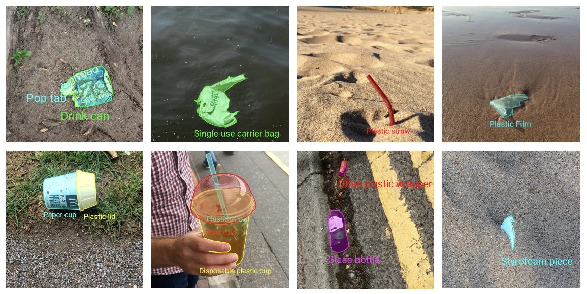
Example images from the official dataset:
About the dataset
- Research Paper: TACO: Trash Annotations in Context for Litter Detection
- Author: Pedro F Proença, Pedro Simões
- Dataset Size: Official: 1500 images, 4784 annotations & Unofficial: 3736 images, 8419 annotations.
- Categories: 60 litter categories
- License: CC BY 4.0
- Release: 17 March 2020
- Read more: Github & Webpage
Downloading the Dataset
So, let’s download the dataset from the official website by following the instructions. Currently, there are two datasets, namely, TACO-Official and TACO-Unofficial.
- The annotations of the official dataset are collected, annotated, and reviewed by the creators of the TACO project.
- The annotations of the unofficial dataset are provided by the community and they are not reviewed.
In this project, we will use the official dataset as a validation set and the unofficial dataset as a training set.
Installing Encord Active
To directly create a conda virtual environment including all packages, check the readme of the project.
Importing the TACO Dataset to Encord Active
You can import a COCO project to Encord Active with a single line command:
encord-active import project --coco -i ./images_folder -a ./annotations.json
We will run the above command twice (once for each dataset). The flow might take a while depending on the performance of your machine, so sit back and enjoy some sweet tunes.
This command will create a local Encord Active project and pre-compute all your quality metrics.
Quality metrics are additional parameterizations added onto your data, labels, and models; they are ways of indexing your data, labels, and models in semantically interesting and relevant ways. In Encord Active, there are different pre-computed metrics that you can use in your projects. You can also write your own custom metrics.
Once the project is imported you will have a local Encord Active project and we can start to understand and analyse the dataset.
Understanding Data and Label Quality
First, let’s analyze the official dataset. To start the Encord Active application, we run the following command for the official dataset:
# from the projects root
encord-active visualise
OR
# from anywhere
encord-active visualise --target /path/to/project/root
Your browser will open a new window with Encord Active.
Data Quality
Now let’s analyze the dataset. First, we navigate to the Data Quality → Explorer tab and check the distribution of samples with respect to different image-level metrics.
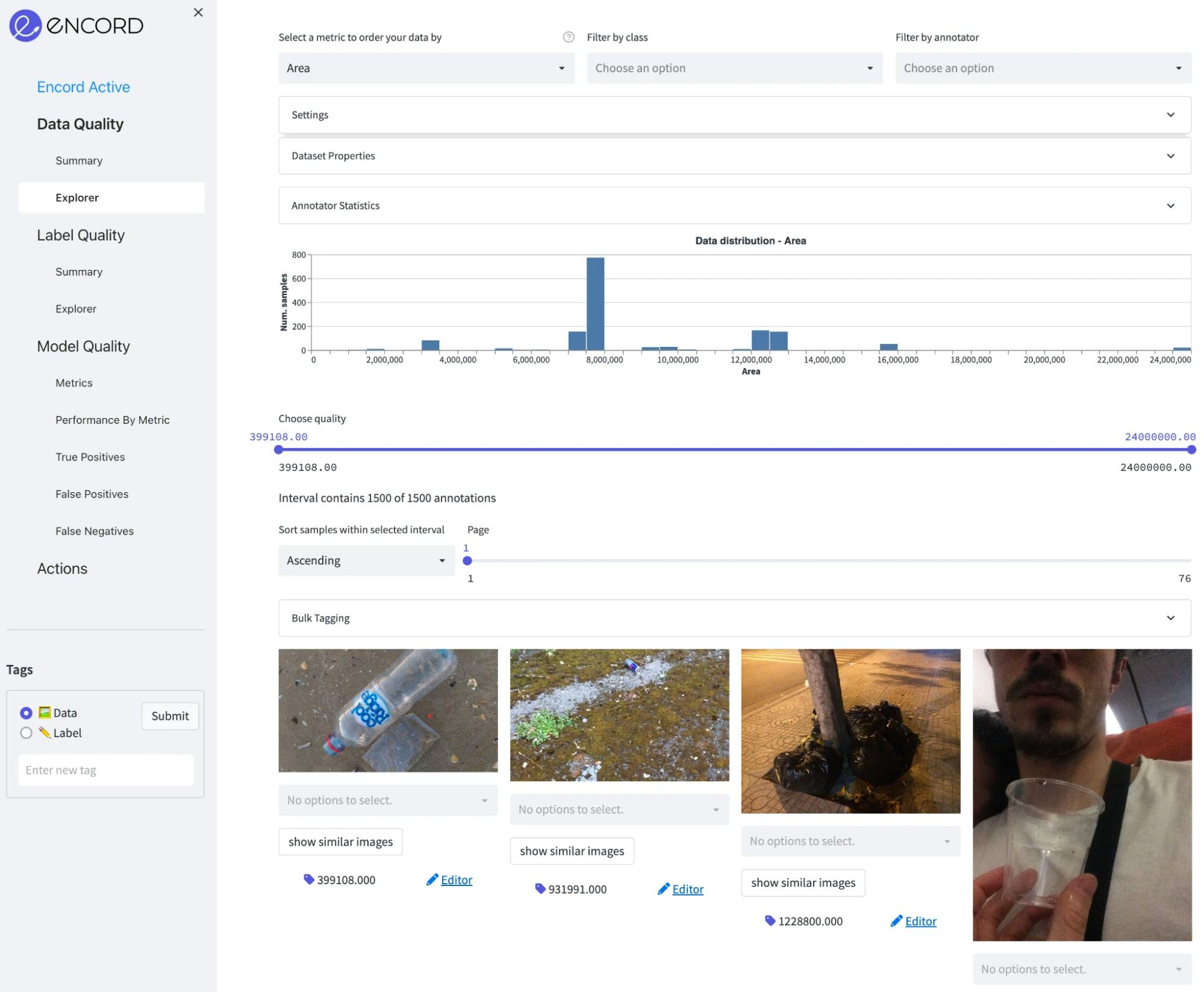
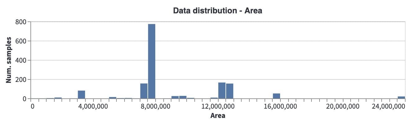
Area: The Images in the dataset are fairly large, where the median image size is around 8 megapixels (roughly 4000x2000). So, they need to be processed properly before the training. Otherwise reading them from the disk will create a serious bottleneck in the data loader. In addition, we can see on the plot below that there are a few outliers of very large images and very small images. Those can be excluded from the dataset.
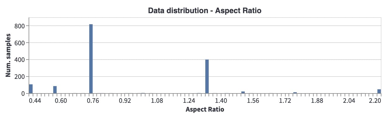
Aspect Ratio: Most images have an aspect ratio of around 0.8, which brings to mind that they are mostly taken with mobile phone cameras (in a vertical direction) which may create a potential bias when going to production.
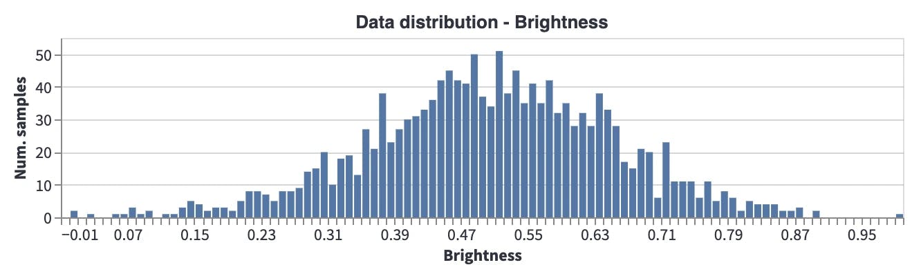
Brightness: Most images are taken during the daytime, and there are a few images taken during the evening (when it is a bit darker). So, this will potentially affect the performance of the model when it is run in environments where it is darker.
Label Quality
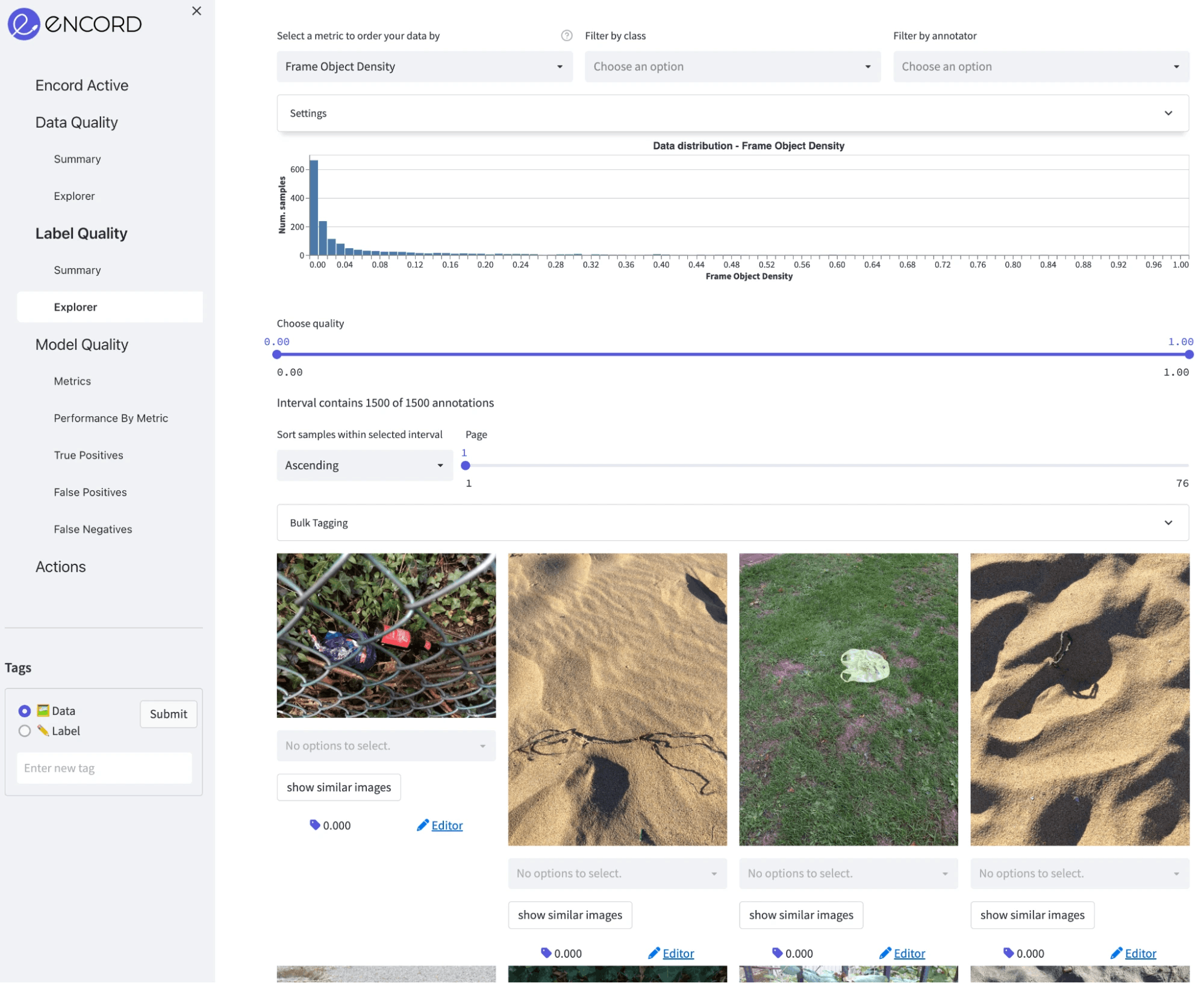
Next, we will analyze the label quality. Go to the Label Quality → Explorer tab and analyze the object-level metrics here:
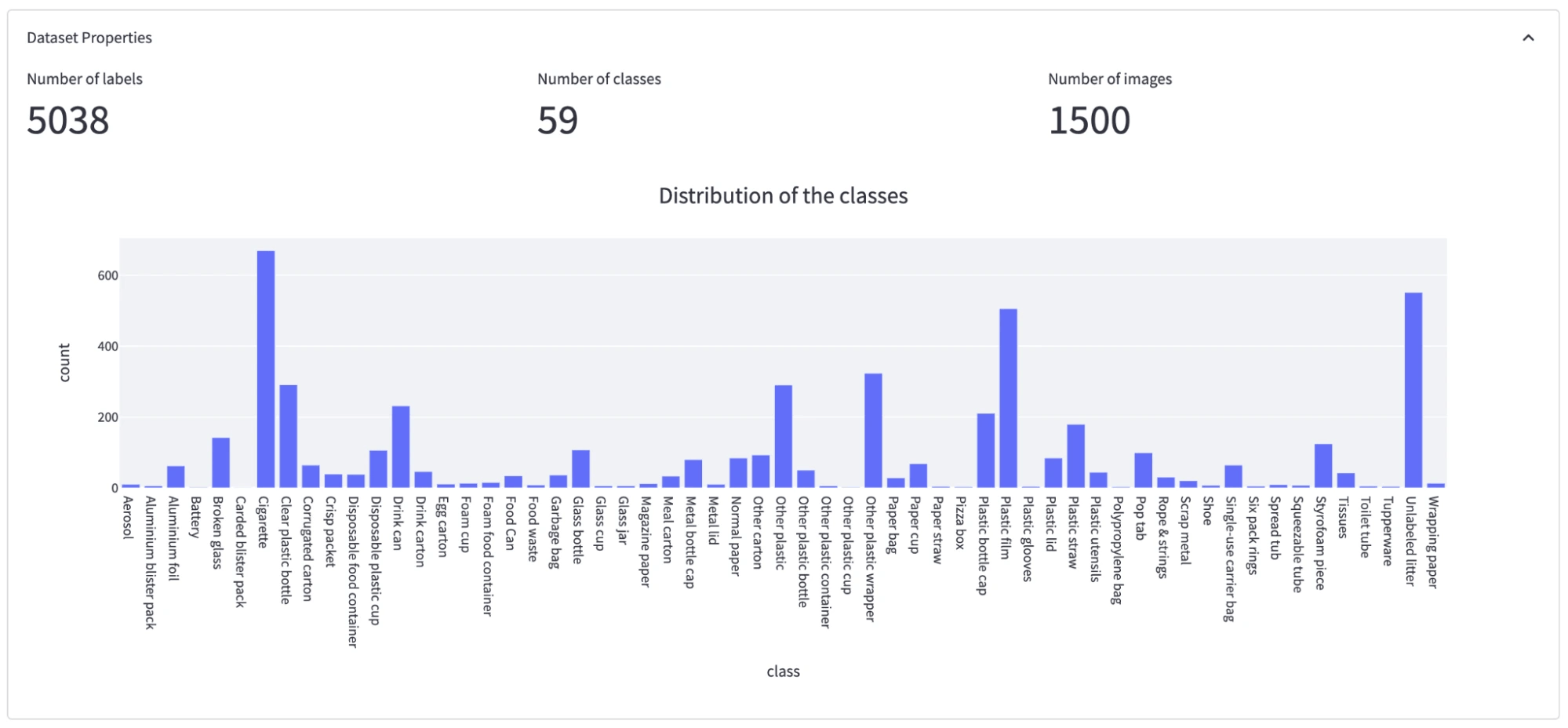
Class distribution: In total, there are 5038 annotations for 59 classes. It is clear that there is a high class imbalance with some classes having fewer than 10 annotations, and some more than 500.
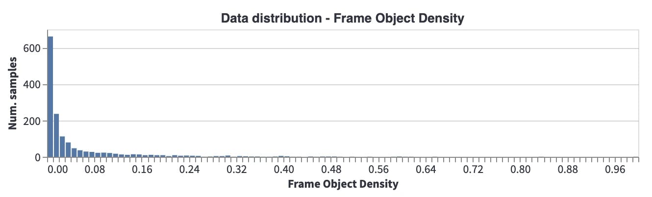
Frame Object Density: In most of the images, objects only cover a small part of the image, which means annotation sizes are small compared to the image size. Thus it is important we choose a model accordingly (AKA avoid using models that have problems with small objects).
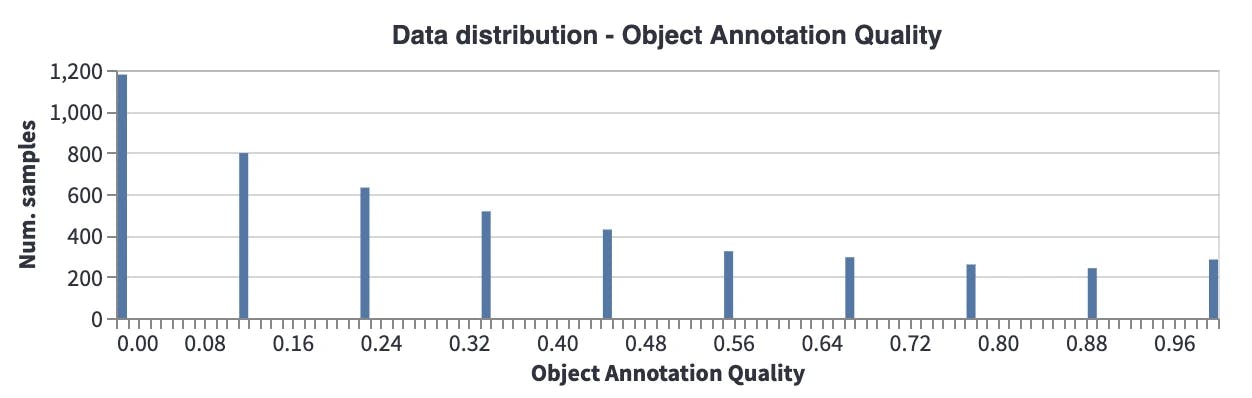
Object Annotation Quality: This metric gives a score for each object according to its closest neighbors in the embedding space. If the closest neighbors have a different label, the quality of the annotation will be low. We see that there are many samples with low object quality scores. This may mean several things: for example, different object classes may be semantically very close to each other, which makes them closer in the embedding space, or there might be annotation errors. These should be analyzed, cleaned, and fixed before model training.
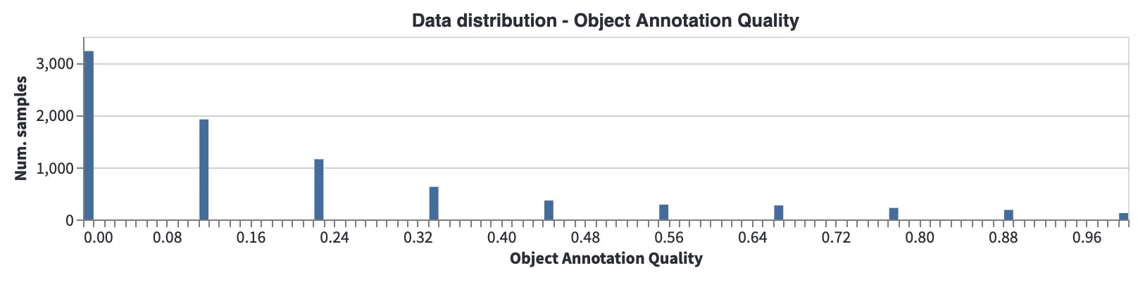
Another interesting point is that when the average object annotation quality scores are compared between the unofficial and official datasets (mean score under Annotator statistics), there is a huge difference (0.195 vs. 0.336). Average scores show that the unofficial dataset has lower annotation quality, so a review of the annotations should be performed before the training.
Distribution of the object annotation quality for the official dataset
Distribution of the object annotation quality for the unofficial dataset
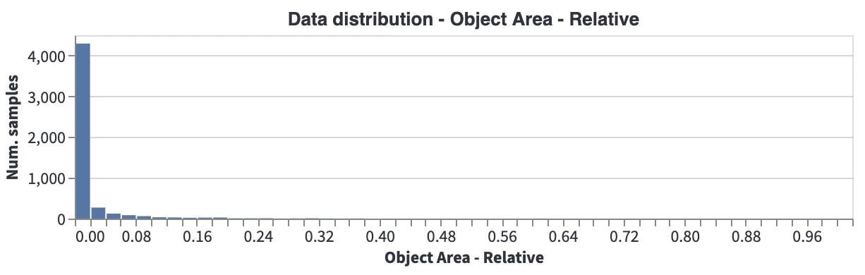
Object Area - Relative: Most of the objects are very small compared to the image. So, for this problem, images can be tiled or frameworks like SAHI can be used.
Takeaways and Insights
Based on the preliminary analysis we can draw following conclusions:
- The images are very large with few outliers, thus we should downsize the images prior to model training and remove the outliers.
- The aspect ratio of most images show that they are probably taken on phone cameras in a vertical perspective. This could potential bias our inference if the edge devices are different.
- A underrepresentation of dark images (night time) can have an effect on our litter detection system at night in a production environment.
- The dataset has a few overrepresented classes (cigarettes, plastic film, unlabeled litter) and many categories with below 20 annotations.
- The annotation quality is significantly worse in the unofficial dataset compared to the official dataset. Whether this is due to label errors or otherwise needs to be investigated.
Next let us start to prepare the data for training :)
Preparing Data for Model Training
First, let’s filter and export the data and annotations to create COCO annotations. Although the datasets already contain COCO annotations, we want to generate a new COCO file where attributes are compatible with Encord Active so when we import our predictions to Encord Active, images can be matched.
- Go to Actions → Filter & Export. Do not filter the data.
- Click Generate COCO file, when COCO file is generated, click Download filtered data to download COCO annotations.
- We perform this operation for both the unofficial and the official dataset.
In every batch, images should be loaded from the disk, however, as we concluded above, they are too large to be loaded efficiently. Therefore, to avoid creating any bottlenecks in our pipeline, we downscale them before starting the training. An example of this can be seen in the project folder utils/downscale_dataset.py. We have scaled all the images to 1024x1024. Loaded images will also be scaled internally by our model before feeding into the model.
Training a Model
For training, we chose to train Mask-RCNN architecture in the Torchvision package. Further, we used PyTorch to train it and Wandb to log the performance metrics.
Create a dataset class
We have implemented EncordMaskRCNNDataset class, which can be used with any COCO dataset generated from the Encord Active so it can be used not just for this project but any project generated from the Encord Active. It transforms the input and output into the format that MaskRCNN model wants:
class EncordMaskRCNNDataset(torchvision.datasets.CocoDetection):
   def __init__(self, img_folder, ann_file, transforms=None):
       super().__init__(img_folder, ann_file)
       self._transforms = transforms

   def __getitem__(self, idx):
       img, target = super().__getitem__(idx)
       img_metadata = self.coco.loadImgs(self.ids[idx])

       image_id = self.ids[idx]
       img_width, img_height = img.size

       boxes, labels, area, iscrowd = [], [], [], []
       for target_item in target:
           boxes.append(
               [
                   target_item["bbox"][0],
                   target_item["bbox"][1],
                   target_item["bbox"][0] + target_item["bbox"][2],
                   target_item["bbox"][1] + target_item["bbox"][3],
               ]
           )

           labels.append(target_item["category_id"])
           area.append(target_item["bbox"][2] * target_item["bbox"][3])
           iscrowd.append(target_item["iscrowd"])

       segmentations = [obj["segmentation"] for obj in target]
       masks = convert_coco_poly_to_mask(segmentations, img_height, img_width)

       processed_target = {}
       processed_target["boxes"] = torch.as_tensor(boxes, dtype=torch.float32)
       processed_target["labels"] = torch.as_tensor(labels, dtype=torch.int64)
       processed_target["masks"] = masks
       processed_target["image_id"] = torch.tensor([image_id])
       processed_target["area"] = torch.tensor(area)
       processed_target["iscrowd"] = torch.as_tensor(iscrowd, dtype=torch.int64)

       if self._transforms is not None:
           img, processed_target = self._transforms(img, processed_target)

       return img, processed_target, img_metadata

   def __len__(self):
       return len(self.ids)
Create data loader
After defining the Torchvision dataset we create a dataset for the data loader:
dataset = EncordMaskRCNNDataset(
   img_folder=params.data.train_data_folder,
   ann_file=params.data.train_ann,
   transforms=get_transform(train=True),
)

data_loader = torch.utils.data.DataLoader(
   dataset,
   batch_size=params.train.batch_size,
   shuffle=True,
   num_workers=params.train.num_worker,
   collate_fn=collate_fn,
)
Create a training loop
The training loop is very straightforward. For each epoch, we train the model on the training set. Once the training is finished for that epoch, we measure the performance on training and validation sets and log the results. To make this training more elegant we have:
- Used a learning rate scheduler to decrease the learning rate when the performance is saturated.
- Used Adam optimizer to quickly converge.
- Only saved the best-performing model checkpoint.
- Used the TorchMetrics library to calculate mAP.
for epoch in range(params.train.max_epoch):
   print(f"epoch: {epoch}")
   train_one_epoch(model, device, data_loader, optimizer, log_freq=10)

   if epoch % params.logging.performance_tracking_interval == 0:
       train_map = evaluate(model, device, data_loader, train_map_metric)
       val_map = evaluate(model, device, data_loader_validation, val_map_metric)

       scheduler.step(val_map["map"])

       if params.logging.wandb_enabled:
           train_map_logs = {f"train/{k}": v.item() for k, v in train_map.items()}
           val_map_logs = {f"val/{k}": v.item() for k, v in val_map.items()}
           wandb.log(
               {
                   "epoch": epoch + 1,
                   "lr": optimizer.param_groups[0]["lr"],
                   **train_map_logs,
                   **val_map_logs,
               }
           )

       val_map_average = val_map["map"].cpu().item()

       if val_map_average > best_map * (1 + 0.0001):
           early_stop_counter = 0
           best_map = val_map_average
           print("overwriting the best model!")

           if params.logging.wandb_enabled:
               wandb.run.summary["best map"] = best_map
               torch.save(
                   model.state_dict(),
                   os.path.join(wandb.run.dir, "best_maskrcnn.ckpt"),
               )
           else:
               torch.save(model.state_dict(), "weights/best_maskrcnn.ckpt")
       else:
           early_stop_counter += 1

       if early_stop_counter >= params.train.early_stopping_thresh:
           print("Early stopping at: " + str(epoch))
           break

print("Training finished")
We have provided the supportive and utility functions and modules inside the project folder.
Before diving into the full model training, let’s check if the training pipeline works as expected. To check that, we run the training on a few samples and expect the model to overfit into those samples. This is a common trick to check if the training pipeline works from end to end as expected.
We have prepared a configuration file (config.ini) to set the training scripts. Once all the paths and training parameters are set correctly, we can start training:
(encord-maskrcnn) > python train.py
Model checkpoints are saved to the local wandb log folder so that we can use it later for inference.
Here is a sample log result for mAP and mAP@50 for both training and validation sets.
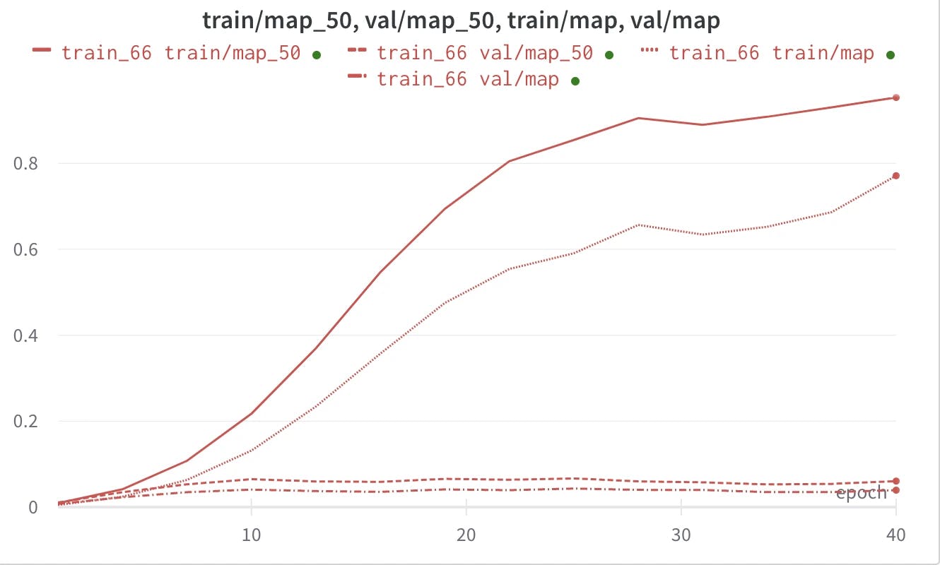
Parameters used for training
- Learning rate = 0.0001
- Batch size = 10
- Epoch = 30
- Num worker = 4
Importing Predictions to Encord Active
There are a few ways to import predictions into Encord Active, for a more detailed explanation please check here.
In this tutorial we will prepare a pickle file consisting of Encord Active Prediction objects, so they can be understood by the Encord Active. First, we need to locate the wandb folder to get the path of the model checkpoint. Every wandb experiment has a unique ID, which can be checked from the overview tab of the experiment on the wandb platform. Once you learned the wandb experiment ID, local checkpoint should be somewhere like this:
/path/to/project/wandb/run-[date_time]_[wandb_id]/files/best_maskrcnn.ckpt
Once you set up the inference section of the config.ini file, you can generate Encord Active predictions.
Here is the main loop to generate the pickle file:
model.eval()
with torch.no_grad():
   for img, _, img_metadata in tqdm(
       dataset_validation, desc="Generating Encord Predictions"
   ):
       prediction = model([img.to(device)])

       scores_filter = prediction[0]["scores"] > confidence_threshold
       masks = prediction[0]["masks"][scores_filter].detach().cpu().numpy()
       labels = prediction[0]["labels"][scores_filter].detach().cpu().numpy()
       scores = prediction[0]["scores"][scores_filter].detach().cpu().numpy()

       for ma, la, sc in zip(masks, labels, scores):
           contours, hierarchy = cv2.findContours(
               (ma[0] > 0.5).astype(np.uint8), cv2.RETR_TREE, cv2.CHAIN_APPROX_NONE
           )
           for contour in contours:
               contour = contour.reshape(contour.shape[0], 2) / np.array(
                   [[ma.shape[2], ma.shape[1]]]
               )
               prediction = Prediction(
                   data_hash=img_metadata[0]["data_hash"],
                   class_id=encord_ontology["objects"][la.item() - 1][
                       "featureNodeHash"
                   ],
                   confidence=sc.item(),
                   format=Format.POLYGON,
                   data=contour,
               )
               predictions_to_store.append(prediction)

with open(
   os.path.join(validation_data_folder, f"predictions_{wandb_id}.pkl"), "wb"
) as f:
   pickle.dump(predictions_to_store, f)
Once we have the pickle file, we run the following command to import predictions:
encord-active import predictions /path/to/predictions.pkl
Lastly, we refresh the Encord Active browser.
Understanding Model Quality
With a freshly trained model, we’re ready to gather some insights. Encord Active automatically matches your ground-truth labels and predictions and presents valuable information regarding the performance of your model. For example:
- mAP performance for different IoU thresholds
- Precision-Recall curve for each class and class-specific AP/AR results
- Which of the 25+ metrics have the highest impact on the model performance
- True positive and false positive predictions as well as false negative ground-truth objects
First we evaluate the model on a high-level.
Model Performance
As explained previously we used the unofficial dataset for the training and official dataset for validation.
For the entire dataset we achieved a mAP @ 0.5 IOU at 0.041.
The mAP is very low. This means that the model is having difficulty detecting litters. We have also trained a model where both training and validation sets are from the official dataset, and the results were around 0.11, which is comparable with the reported results in the literature. This result also shows how difficult our task is.
Important Quality Metrics
First we want to investigate what quality metrics impact model performance. High importance for a metric implies that a change in that quantity would strongly affect model performance:
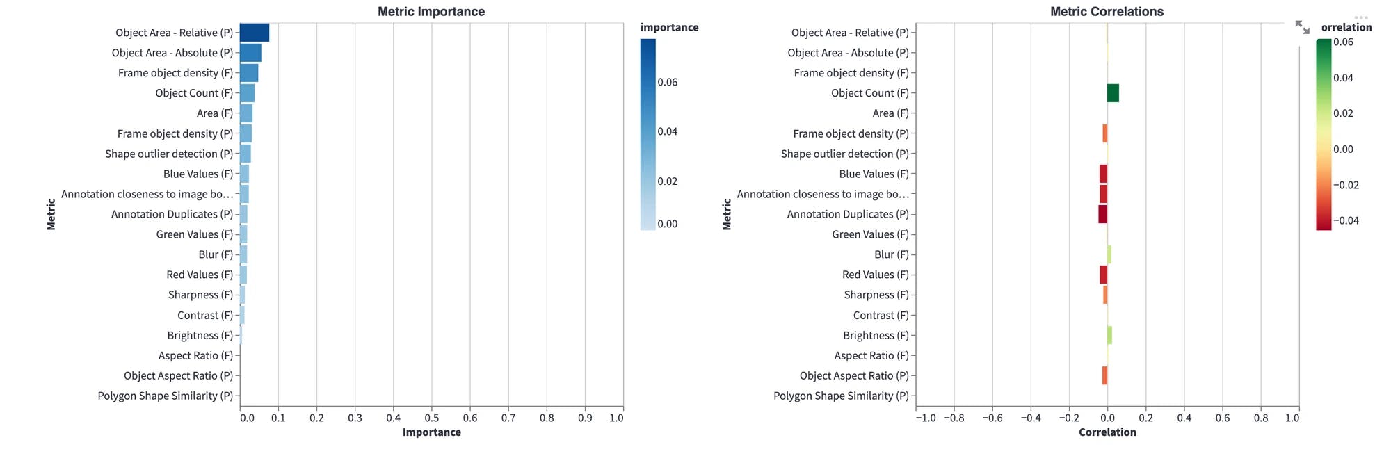
Hmm... object area, frame object density, and object count are most important metrics for the model performance. We should investigate that.
Best performing objects
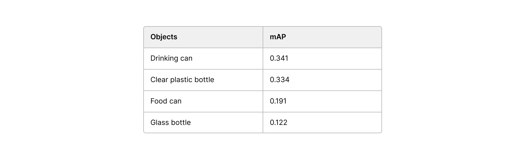
Not surprisingly, among the best performing object are larger and distinct object such as cans and bottles.
Worst performing objects

Worst performing objects are the ones which do not have a clear definition: other plastic, other cartoon, unlabeled litter.
Other model insights
Next we, go dive into the model performance by metric and examine performance with respect to different metrics. Here are some insights we got from there:
- False negative rate and object count (number of labels pr. image) are directly proportional.
- The model tends to miss ground-truth objects when the sharpness value of the image is low (Image is more blurry).
- The smaller an object is relative to the image the worse performance. This is especially true for objects whose area are less than 0.01% of the image.
True positives
Let’s examine a few true positive:
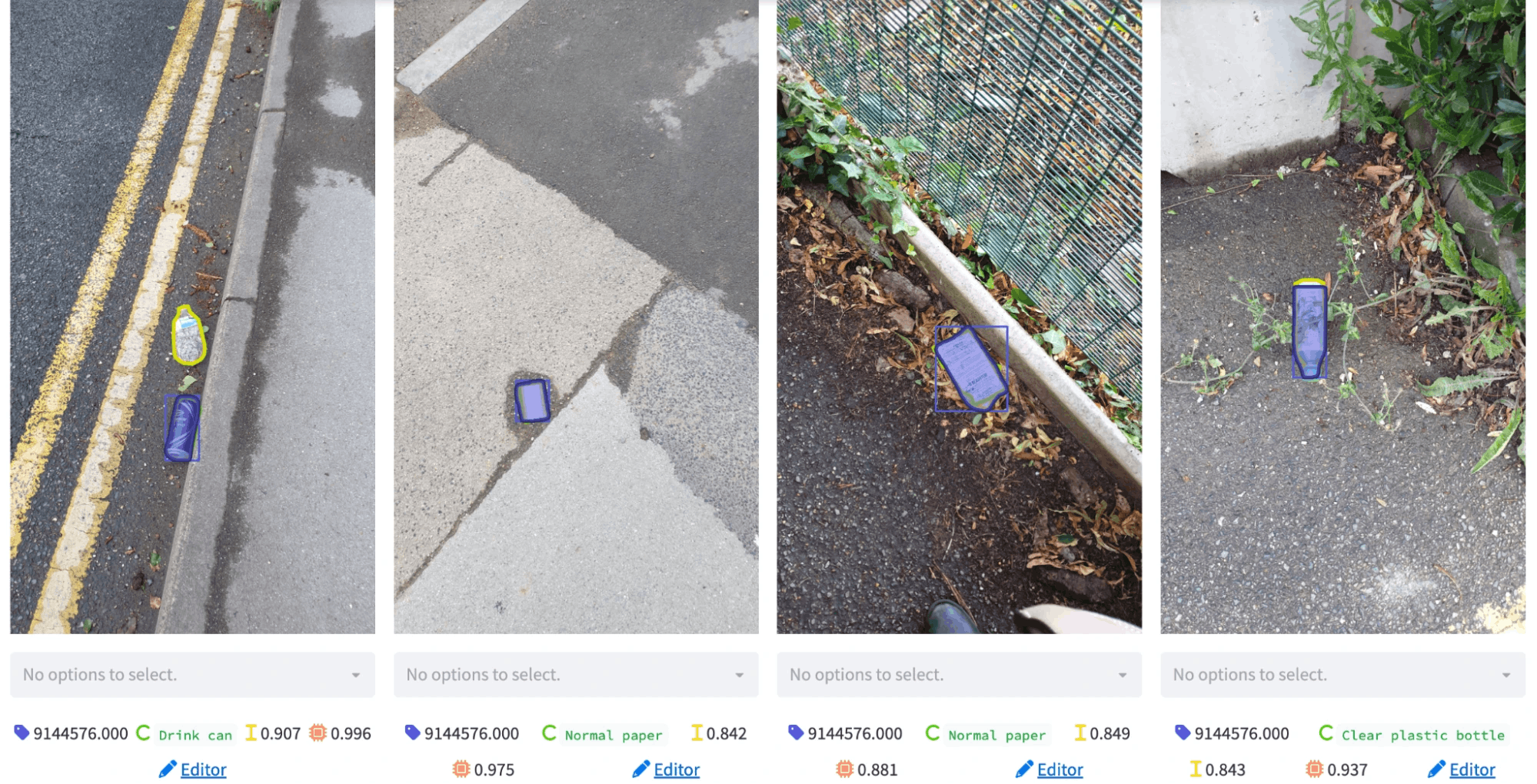
The model segments some objects very well. In this tab, we can rank all true positives according to a metric that we want. For example, if we want to visualize correctly segmented objects in small images, we can select the area metric on the top bar.
False positives
Let’s examine a few false positives:
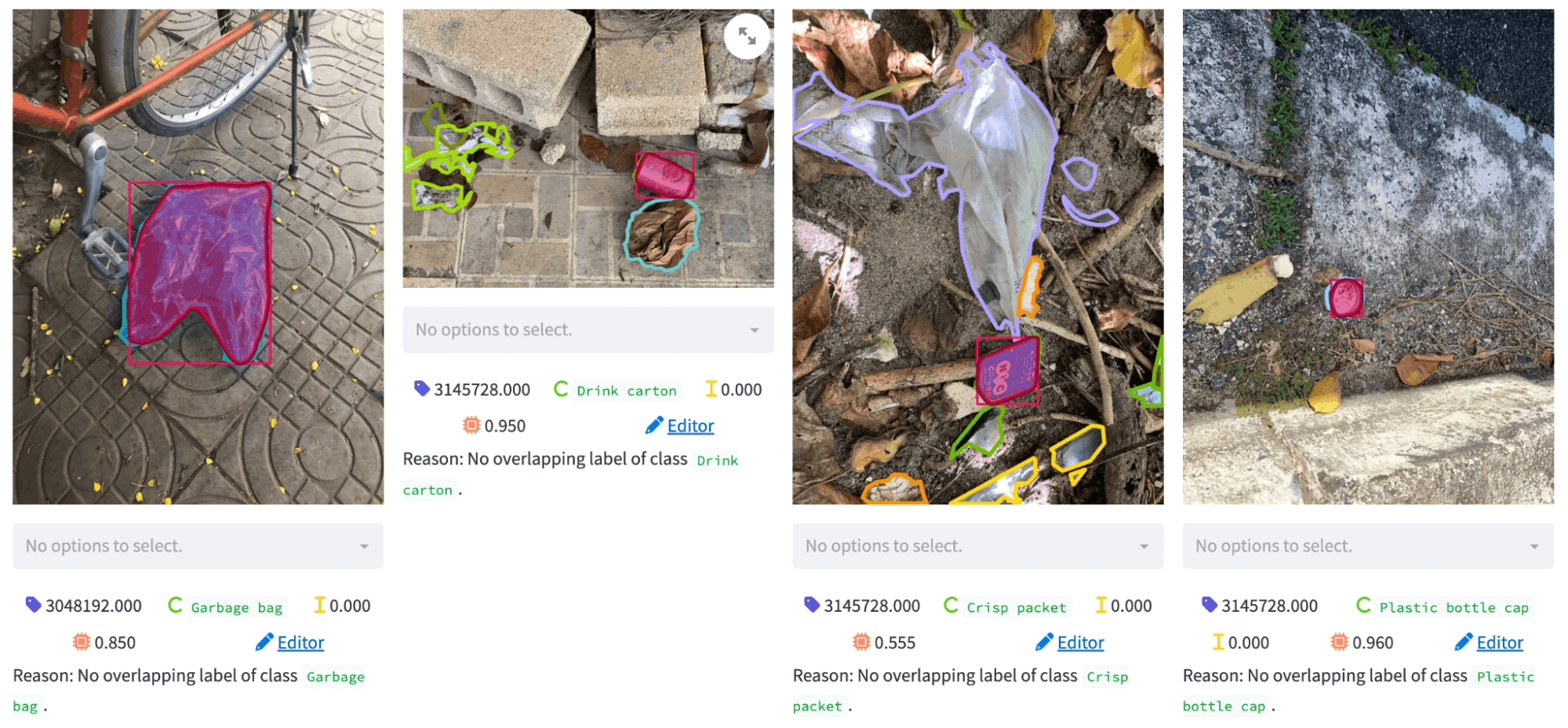
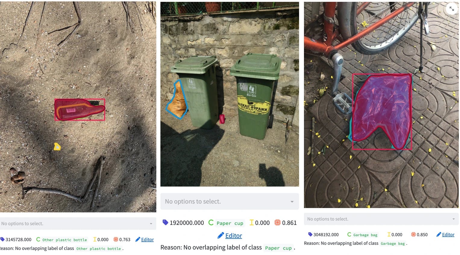
We see some interesting patterns here. The model’s segmentation for the objects are quite good, however, they are regarded as false positives. This may mean two things: 1) the model is confused about the object class or 2) there is a missing annotation. After inspecting the ground truth labels, we found that there are some classes which are confused with each other (e.g., garbage bag vs. single use carrier bag, glass bottle vs. other plastic bottle).
Examples from picture below
- The glass bottle is detected as other plastic bottle.
- The paper cup has no ground truth annotation:
- The single use carrier bag is perfectly detected as a garbage bag.
If we detect frequently confused objects, we can provide more data for these object classes or we can add specific post-processing steps to our inference pipeline, which will eventually increase our overall performance. These points are all very valuable to know when building our litter detection system since they show us areas we need improvement in our computer vision pipeline.
Conclusion
With the help of the Encord Active, we now have a better understanding of what we have in our hands and we:
- Obtained useful information on images such as their area, aspect ratio, brightness levels, which might be useful in building the training pipeline.
- Inspected class distribution and learned that there is a high class imbalance.
- Found that most of the objects are very small. In addition, the annotation quality of the crowd-sourced dataset is a lot worse than the official dataset; therefore, annotations should be reviewed.
- Inspected overall and class-based performance metrics. We learned that object area, frame object density, and object count have the highest impact on performance over others, and thus we should pay attention to those when retraining the model.
- Visualized true positives and false positive samples and figured out that there is a class mismatch problem. If this is solved, it will significantly reduce the false negatives.
Further Steps
With the insights we got from Encord Active, we now know what should be prioritized. In the second part of this tutorial, we will utilize the information we obtained here to improve our baseline result with a new and improved dataset.
Want to test your own models?
"I want to get started right away" - You can find Encord Active on Github here.
"Can you show me an example first?" - Check out this Colab Notebook.
"I am new, and want a step-by-step guide" - Try out the getting started tutorial.
If you want to support the project you can help us out by giving a Star on GitHub :)
Want to stay updated?
- Follow us on Twitter and Linkedin for more content on computer vision, training data, and active learning.
- Join the Slack community to chat and connect.
Explore our products
Index
Manage & curate your data
Understand and manage your visual data, prioritize data for labeling, and initiate active learning pipelines.

Annotate
Supporting your labeling needs
Super charge your data annotation with AI-powered labeling — including automated interpolation, object detection and ML-based quality control.

Active
Find & fix data issues with ease
Monitor, troubleshoot, and evaluate the data and labels impacting model performance.