
Insights for AI Builders
Encord Blog
All articles
423 of 423 articles
How to annotate video for machine learning: A Step-by-Step workflow
Video Annotation
Jul 13 2026
You Don't Have a Data Problem. You Have a Curation Problem
Data Curation
Jul 10 2026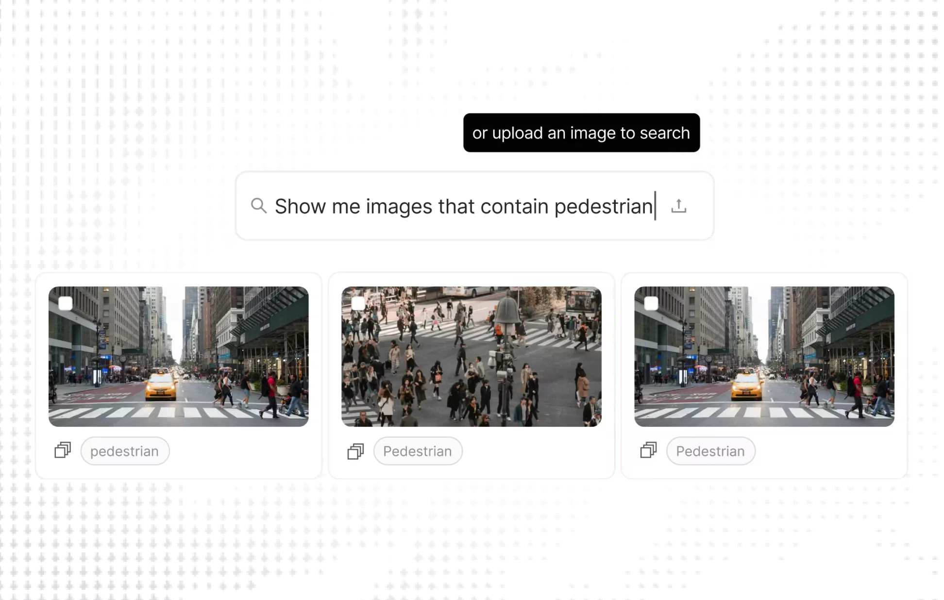
AI Data Curation for LLM and Multimodal Teams: A Practical Framework
Data Curation
Jul 09 2026
Data Curation Best Practices for AI: A Step-by-Step Framework
Data Curation
Jul 09 2026
What Is Data Curation? The Complete Guide
Data Curation
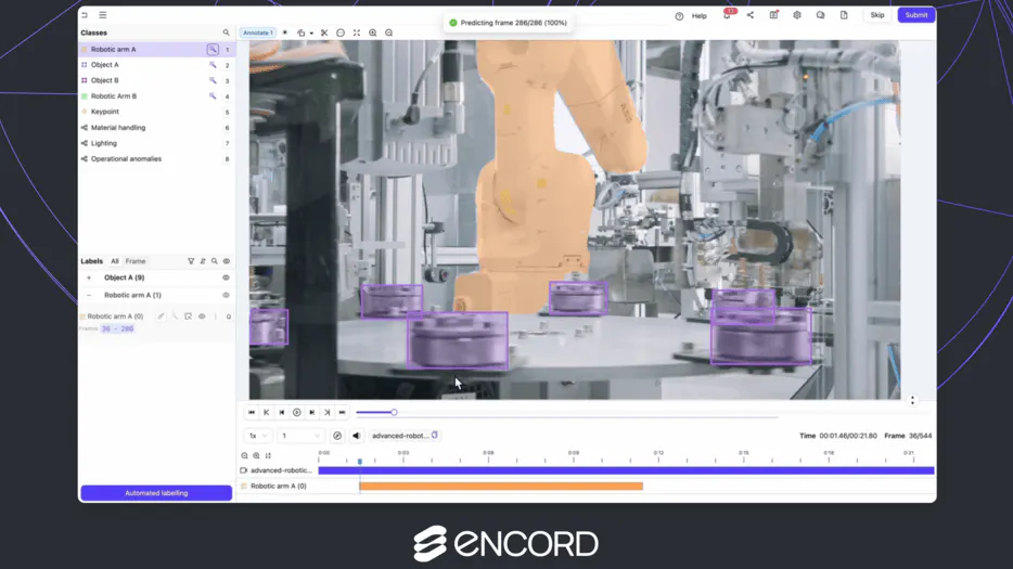
Jul 08 2026![[Webinar Recap] How NVIDIA Cosmos 3 Is Changing the Way Physical AI Teams Build Training Data](https://images.prismic.io/encord/GV2SxWuhLGm0vpTQ_NVIDIAcosmoswebianrbanner-1-copy2.png?auto=format%2Ccompress&fit=max)
[Webinar Recap] How NVIDIA Cosmos 3 Is Changing the Way Physical AI Teams Build Training Data
Agents
Jul 07 2026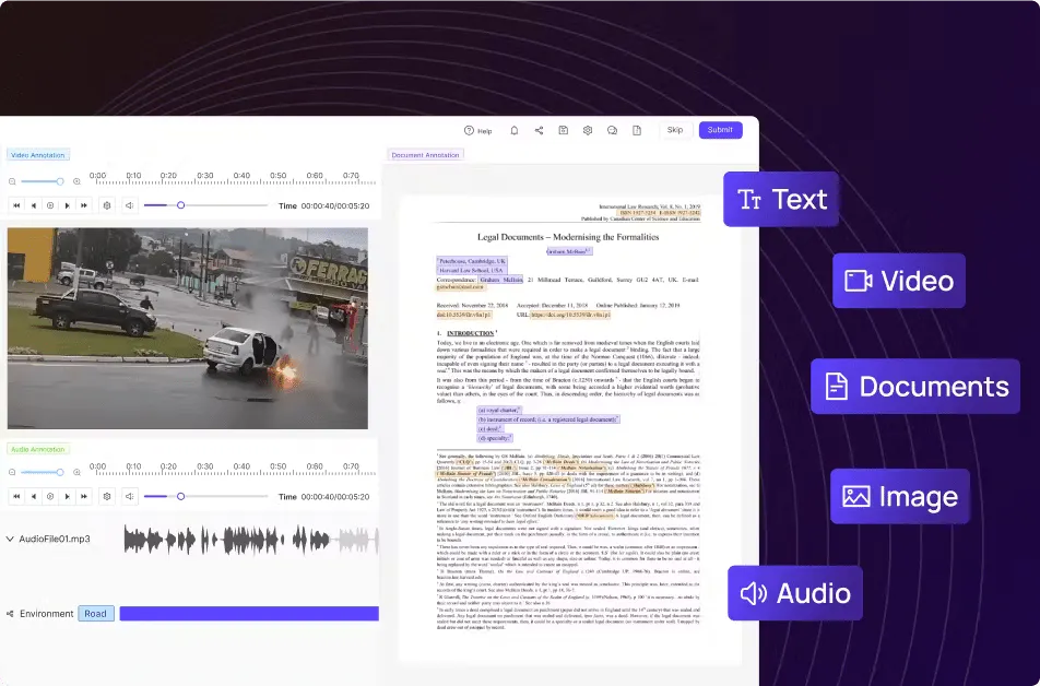
Multimodal Data Labeling: One Pipeline for Image, Video, Audio, Text and 3D
Data Annotation
Jul 07 2026
What Is AI Data Labeling? Definition, Types and the Process
Data Annotation
Jul 07 2026
Build vs buy: A decision framework for data labeling tools
Data Annotation
Jul 06 2026
Data Labeling Quality Control: Consensus, Inter-Annotator Agreement and QA Workflows
Data Quality
Jul 06 2026
How to Label Data for Machine Learning: A Step-by-Step Workflow
Machine Learning
Jul 02 2026
Introducing Merlin: The Agentic Intelligence Layer for Encord
Agents
Jun 16 2026