YOLO Object Detection Explained: Evolution, Algorithm, and Applications

Product Manager at Encord
What is YOLO Object Detection?
YOLO (You Only Look Once) models are real-time object detection systems that identify and classify objects in a single pass of the image. In other words, the model only looks at the image once and from this ‘single pass’ is able to identify objects in the image. This is different from previous models that required multiple passes to process an image. Since this process happens in real-time, it works at incredible speed.
Object detection means that YOLO can not only pinpoint where an object is in an image but also what it is. This works by passing the image through a neural network that allows the model to detect all objects simultaneously. Using grid-based prediction and bounding box prediction, the model is able to understand if objects fall within a certain cell or bounding box. Additionally, YOLO uses class probability to predict how to classify objects, which determines what the object actually is.
YOLO has a number of advantages in comparison to previous methods. As mentioned, it is extremely fast and can therefore be applied to use chases such as self-driving cars and video surveillance. Additionally, it has high accuracy, especially with natural images, and fewer false positives since it analyzes an entire image at once, which provides greater contextual accuracy.
What is Object Detection?
Object detection is a critical capability of computer vision that identifies and locates objects within an image or video. Unlike image classification, object detection not only classifies the objects in an image, but also identifies their location within the image by drawing a bounding box around each object. Object detection models, such as R-CNN, Fast R-CNN, Faster R-CNN, and YOLO, use convolutional neural networks (CNNs) to classify the objects and regressor networks to accurately predict the bounding box coordinates for each detected object.
Image Classification
Image classification is a fundamental task in computer vision. Given an input image, the goal of an image classification model is to assign it to one of a pre-defined set of classes. Most image classification models use CNNs, which are specifically designed to process pixel data and can capture spatial features. Image classification models are trained on large datasets (like ImageNet) and can classify images into 1000 object categories, such as keyboard, mouse, pencil, and many animals.
Object Localization
Object localization is another important task in computer vision that identifies the location of an object in the image. It extends the image classification model by adding a regression head to predict the bounding box coordinates of the object. The bounding box is typically represented by four coordinates that define its position and size. Object localization is a key step in object detection, where the goal is not just to classify the primary object of interest in the image, but also to identify its location.
Classification of Object Detection Algorithms
Object detection algorithms can be broadly classified into two categories: single-shot detectors and two-shot(or multi-shot) detectors. These two types of algorithms have different approaches to the task of object detection.
Single-Shot Object Detection
Single-shot detectors (SSDs) are a type of object detection algorithm that predict the bounding box and the class of the object in one single shot. This means that in a single forward pass of the network, the presence of an object and the bounding box are predicted simultaneously. This makes SSDs very fast and efficient, suitable for tasks that require real-time detection.
Examples of single-shot object detection algorithms include YOLO (You Only Look Once) and SSD (Single Shot MultiBox Detector). YOLO divides the input image into a grid and for each grid cell, predicts a certain number of bounding boxes and class probabilities. SSD, on the other hand, predicts bounding boxes and class probabilities at multiple scales in different feature maps.
Two-Shot Object Detection
Two-shot or multi-shot object detection algorithms, on the other hand, use a two-step process for detecting objects. The first step involves proposing a series of bounding boxes that could potentially contain an object. This is often done using a method called region proposal. The second step involves running these proposed regions through a convolutional neural network to classify the object classes within the box.
Examples of two-shot object detection algorithms include R-CNN (Regions with CNN features), Fast R-CNN, and Faster R-CNN. These algorithms use region proposal networks (RPNs) to propose potential bounding boxes and then use CNNs to classify the proposed regions.
Both single-shot and two-shot detectors have their strengths and weaknesses. Single-shot detectors are generally faster and more efficient, making them suitable for real-time object detection tasks. Two-shot detectors, while slower and more computationally intensive, tend to be more accurate, as they can afford to spend more computational resources on each potential object.
Object Detection Methods
Object Detection: Non-Neural Methods
Viola-Jones object detection method based on Haar features
The Viola-Jones method, introduced by Paul Viola and Michael Jones, is a machine learning model for object detection. It uses a cascade of classifiers, selecting features from Haar-like feature sets. The algorithm has four stages:
- Haar Feature Selection
- Creating an Integral Image
- Adaboost Training
- Cascading Classifiers
Despite its simplicity and speed, it can achieve high detection rates.
Scale-Invariant Feature Transform (SIFT)
SIFT is a method for extracting distinctive invariant features from images. These features are invariant to image scale and rotation, and are robust to changes in viewpoint, noise, and illumination. SIFT features are used to match different views of an object or scene.
Histogram of Oriented Gradients (HOG)
HOG is a feature descriptor used for object detection in computer vision. It involves counting the occurrences of gradient orientation in localized portions of an image. This method is similar to edge orientation histograms, scale-invariant feature transform descriptors, and shape contexts, but differs in that it is computed on a dense grid of uniformly spaced cells.
Object Detection: Neural Methods
Region-Based Convolutional Neural Networks (R-CNN)
Region-Based CNN uses convolutional neural networks to classify image regions in order to detect objects. It involves training a CNN on a large labeled dataset and then using the trained network to detect objects in new images. Region-Based CNN and its successors, Fast R-CNN and Faster R-CNN, are known for their accuracy but can be computationally intensive.
Faster R-CNN
Faster R-CNN is an advanced version of R-CNN that introduces a Region Proposal Network (RPN) for generating region proposals. The RPN shares full-image convolutional features with the detection network, thus enabling nearly cost-free region proposals. The RPN is a fully convolutional network that simultaneously predicts object bounds and objectness scores at each position. Faster R-CNN is faster than the original R-CNN and Fast R-CNN because it doesn’t need to run a separate region proposal method on the image, which can be slow.
Mask R-CNN
Mask R-CNN extends Faster R-CNN by adding a branch for predicting an object mask in parallel with the existing branch for bounding box recognition. This allows Mask R-CNN to generate precise segmentation masks for each detected object, in addition to the class label and bounding box. The mask branch is a small fully convolutional network applied to each RoI, predicting a binary mask for each RoI. Mask R-CNN is simple to train and adds only a small computational overhead, enabling a fast system and rapid experimentation.
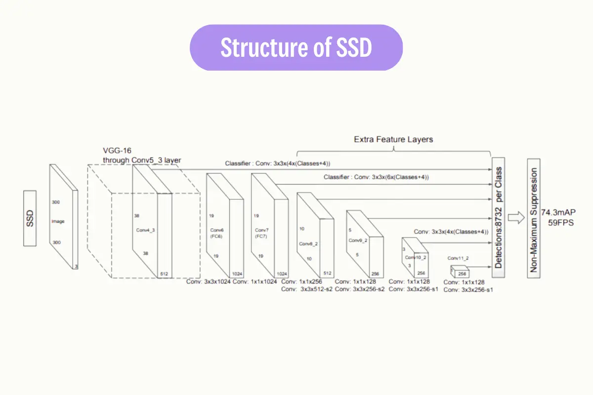
Single Shot Detector (SSD)
SSD is a method for object detection that eliminates the need for multiple network passes for multiple scales. It discretizes the output space of bounding boxes into a set of default boxes over different aspect ratios and scales per feature map location. SSD is faster than methods like R-CNN because it eliminates bounding box proposals and pooling layers.
RetinaNet
RetinaNet uses a feature pyramid network on top of a backbone to detect objects at different scales and aspect ratios. It introduces a new loss, the Focal Loss, to deal with the foreground-background class imbalance problem. RetinaNet is designed to handle dense and small objects.
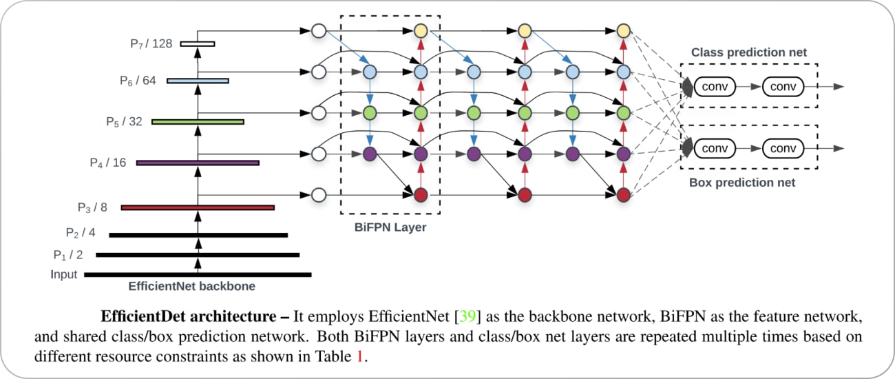
EfficientDet
EfficientDet is a method that scales all dimensions of the network width, depth, and resolution with a compound scaling method to achieve better performance. It introduces a new architecture, called BiFPN, which allows easy and efficient multi-scale feature fusion, and a new scaling method that uniformly scales the resolution, depth, and width for all backbone, feature network, and box/class prediction networks at the same time. EfficientDet achieves state-of-the-art accuracy with fewer parameters and less computation compared to previous detectors.
You Only Look Once (YOLO)
YOLO, developed by Joseph Redmon et al., frames object detection as a regression problem to spatially separated bounding boxes and associated class probabilities. It looks at the whole image at test time so its predictions are informed by global context in the image. YOLO is known for its speed, making it suitable for real-time applications.
You Only Look Once: Unified, Real-Time Object Detection
Object Detection: Performance Evaluation Metrics
Intersection over Union (IoU)

IoU (Intersection over Union) Calculation
Intersection over Union (IoU) is a common metric used to evaluate the performance of an object detection algorithm. It measures the overlap between the predicted bounding box (P) and the ground truth bounding box (G). The IoU is calculated as the area of intersection divided by the area of union of P and G.
The IoU score ranges from 0 to 1, where 0 indicates no overlap and 1 indicates a perfect match. A higher IoU score indicates a more accurate object detection.
Average Precision (AP)
Average Precision (AP) is another important metric used in object detection. It summarizes the precision-recall curve that is created by varying the detection threshold.
Precision is the proportion of true positive detections among all positive detections, while recall is the proportion of true positive detections among all actual positives in the image.
The AP computes the average precision values for recall levels over 0 to 1. The AP score ranges from 0 to 1, where a higher value indicates better performance. The mean Average Precision (mAP) is often used in practice, which calculates the AP for each class and then takes the average.
By understanding these metrics, we can better interpret the performance of models like YOLO and make informed decisions about their application in real-world scenarios.
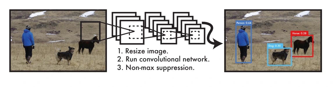
After exploring various object detection methods and performance evaluation methods, let’s delve into the workings of a particularly powerful and popular algorithm known as ‘You Only Look Once’, or YOLO. This algorithm has revolutionized the field of object detection with its unique approach and impressive speed.
Unlike traditional methods that involve separate steps for identifying objects and classifying them, YOLO accomplishes both tasks in a single pass, hence the name ‘You Only Look Once’.
YOLO Object Detection Algorithm: How Does it Work?
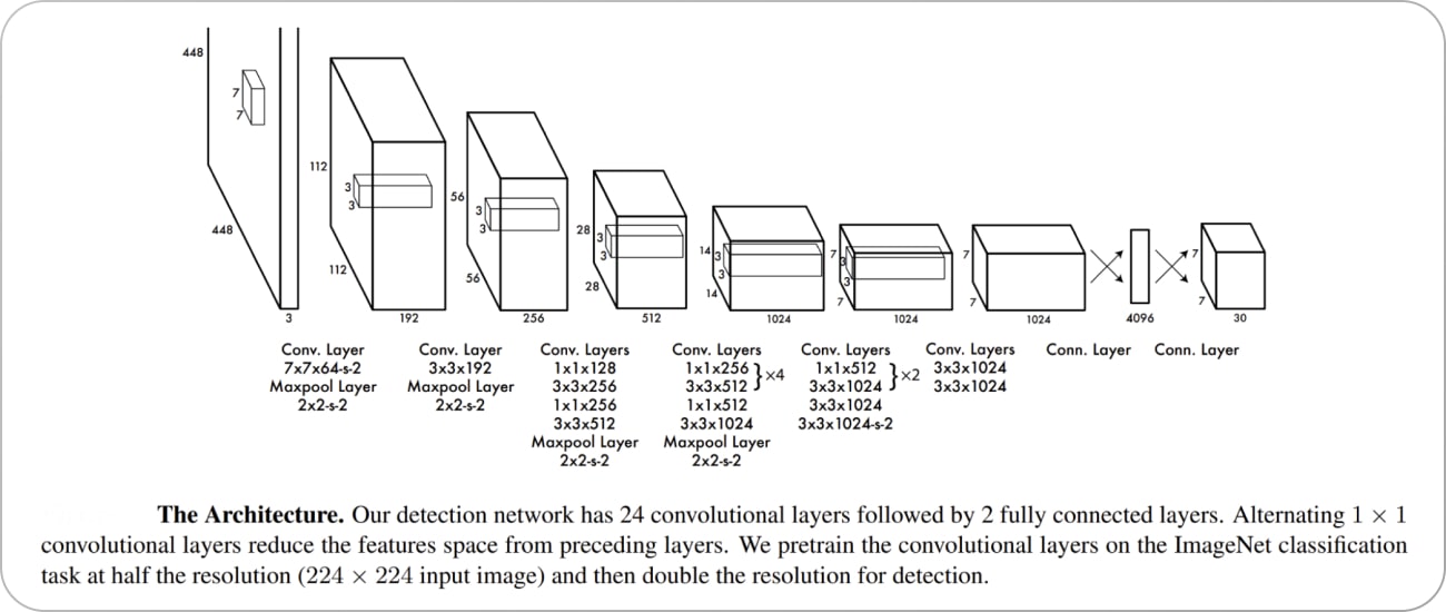
YOLO Architecture
The YOLO algorithm employs a single Convolutional Neural Network (CNN) that divides the image into a grid. Each cell in the grid predicts a certain number of bounding boxes. Along with each bounding box, the cell also predicts a class probability, which indicates the likelihood of a specific object being present in the box.
Bounding Box Recognition Process
The bounding box recognition process in YOLO involves the following steps:
- Grid Creation: The image is divided into an SxS grid. Each grid cell is responsible for predicting an object if the object’s center falls within it.
- Bounding Box Prediction: Each grid cell predicts B bounding boxes and confidence scores for those boxes. The confidence score reflects how certain the model is that a box contains an object and how accurate it thinks the box is.
- Class Probability Prediction: Each grid cell also predicts C conditional class probabilities (one per class for the potential objects). These probabilities are conditioned on there being an object in the box.
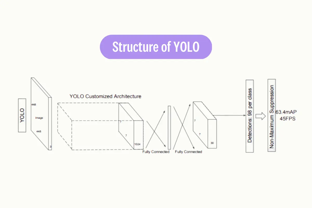
Non-Max Suppression (NMS)
After the bounding boxes and class probabilities are predicted, post-processing steps are applied. One such step is Non-Max Suppression (NMS). NMS helps in reducing the number of overlapping bounding boxes. It works by eliminating bounding boxes that have a high overlap with the box that has the highest confidence score.
Vector Generalization
Vector generalization is a technique used in the YOLO algorithm to handle the high dimensionality of the output. The output of the YOLO algorithm is a tensor that contains the bounding box coordinates, objectness score, and class probabilities.
This high-dimensional tensor is flattened into a vector to make it easier to process. The vector is then passed through a softmax function to convert the class scores into probabilities. The final output is a vector that contains the bounding box coordinates, objectness score, and class probabilities for each grid cell.

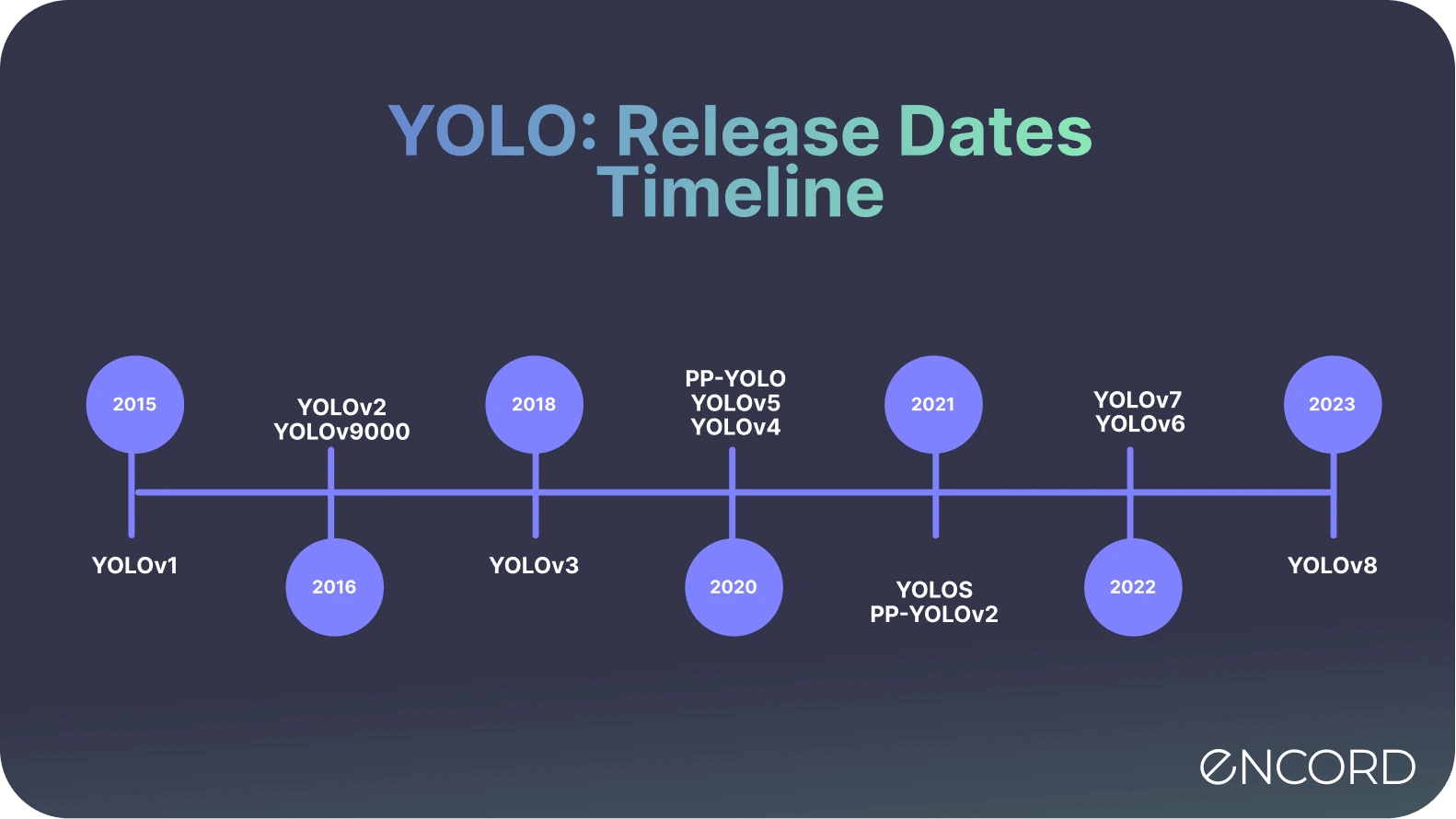
Evolution of YOLO: YOLOv1, YOLOv2, YOLOv3, YOLOv4, YOLOR, YOLOX, YOLOv5, YOLOv6, YOLOv7, YOLOv8, YOLOv9
If you are not interested in a quick recap of the timeline of YOLO models and the updates in the network architecture, skip this section!
YOLOv1: First Real-time Object Detection Algorithm
The original YOLO model treated object detection as a regression problem, which was a significant shift from the traditional classification approach. It used a single convolutional neural network (CNN) to detect objects in images by dividing the image into a grid, making multiple predictions per grid cell, filtering out low-confidence predictions, and then removing overlapping boxes to produce the final output.
YOLOv2 [YOLO9000]: Multi-Scale Training| Anchor Boxes| Darknet-19 Backbone
YOLOv2 introduced several improvements over the original YOLO. It used batch normalization in all its convolutional layers, which reduced overfitting and improved model stability and performance. It could handle higher-resolution images, making it better at spotting smaller objects. YOLOv2 also used anchor boxes (borrowed from Faster R-CNN), which helped the algorithm predict the shape and size of objects more accurately.
YOLOv3: Three YOLO Layers| Logistic Classifiers| Upsampling |Darknet-53 Backbone
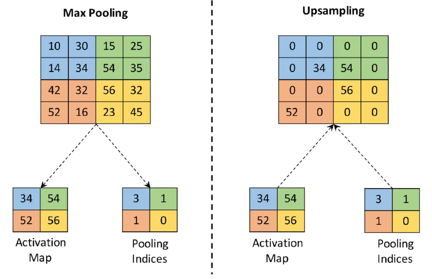
YOLOv3 introduced a new backbone network, Darknet-53, which utilized residual connections. It also made several design changes to improve accuracy while maintaining speed. At 320x320 resolution, YOLOv3 ran in 22 ms at 28.2 mAP, as accurate as SSD but three times faster. It achieved 57.9 mAP@50 in 51 ms on a Titan X, compared to 57.5 mAP@50 in 198 ms by RetinaNet, with similar performance but 3.8x faster.
YOLOv4: CSPDarknet53 | Detection Across Scales | CIOU Loss
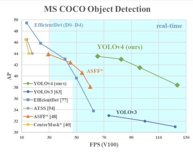
Speed Comparison: YOLOv4 Vs. YOLOv3
YOLOv4 introduced several new techniques to improve both accuracy and speed. It used a CSPDarknet backbone and introduced new techniques such as spatial attention, Mish activation function, and GIoU loss to improve accuracy3. The improved YOLOv4 algorithm showed a 0.5% increase in average precision (AP) compared to the original algorithm while reducing the model’s weight file size by 45.3 M.
YOLOR: Unified Network Architecture | Mosaic | Mixup | SimOTA

UNA (Unified Network Architecture)
Unlike previous YOLO versions, YOLOR’s architecture and model infrastructure differ significantly. The name “YOLOR” emphasizes its unique approach: it combines explicit and implicit knowledge to create a unified network capable of handling multiple tasks with a single input. By learning just one representation, YOLOR achieves impressive performance in object detection.
YOLOX
YOLOX is an anchor-free object detection model that builds upon the foundation of YOLOv3 SPP with a Darknet53 backbone. It aims to surpass the performance of previous YOLO versions. The key innovation lies in its decoupled head and SimOTA approach. By eliminating anchor boxes, YOLOX simplifies the design while achieving better accuracy. It bridges the gap between research and industry, offering a powerful solution for real-time object detection. YOLOX comes in various sizes, from the lightweight YOLOX-Nano to the robust YOLOX-x, each tailored for different use cases.
YOLOv5: PANet| CSPDarknet53| SAM Block
YOLOv5 brought about further enhancements to increase both precision and efficiency. It adopted a Scaled-YOLOv4 backbone and incorporated new strategies such as CIOU loss and CSPDarknet53-PANet-SPP to boost precision.
The refined YOLOv5 algorithm demonstrated a 0.7% rise in mean average precision (mAP) compared to the YOLOv4, while decreasing the model’s weight file size by 53.7 M. These improvements made YOLOv5 a more effective and efficient tool for real-time object detection.
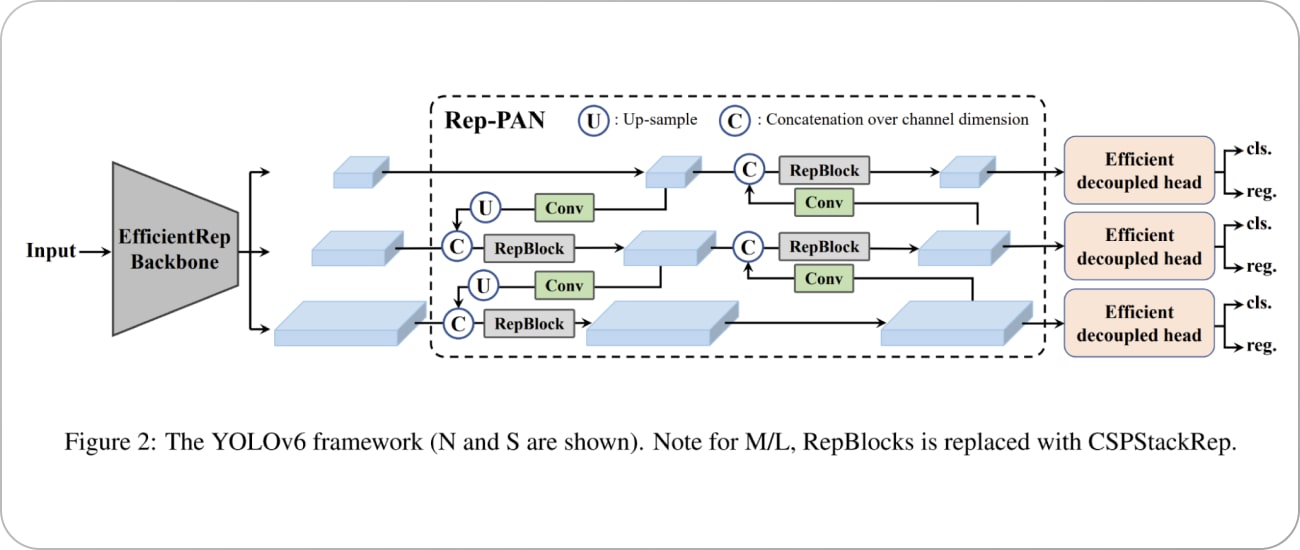
YOLOv6: EfficientNet-Lite | CSPDarknet-X backbone | Swish Activation Function | DIoU Loss
YOLOv6 utilized a CSPDarknet-X backbone and introduced new methods such as panoptic segmentation, Swish activation function, and DIoU loss to boost accuracy.
The enhanced YOLOv6 algorithm exhibited a 0.8% increase in average precision (AP) compared to the YOLOv5, while shrinking the model’s weight file size by 60.2 M. These advancements made YOLOv6 an even more powerful tool for real-time object detection.
YOLOv7: Leaky ReLU Activation Function| TIoU Loss| CSPDarknet-Z Backbone
YOLOv7 employed a CSPDarknet-Z backbone in the yolov7 architecture. YOLOv7 object detection algorithm was enhanced by the introduction of innovative techniques such as object-centric segmentation, Leaky ReLU activation function, and TIoU loss to enhance accuracy.

The advanced YOLOv7 algorithm demonstrated a 1.0% increase in average precision (AP) compared to the YOLOv6, while reducing the model’s weight file size by 70.5 M. These improvements made YOLOv7 object detection algorithm, an even more robust tool for real-time object detection.
YOLOv8: Multi-Scale Object Detection| CSPDarknet-AA| ELU Activation Function| GIoU Loss
YOLOv8 introduced a new backbone architecture, the CSPDarknet-AA, which is an advanced version of the CSPDarknet series, known for its efficiency and performance in object detection tasks.
One key technique introduced in YOLOv8 is multi-scale object detection. This technique allows the model to detect objects of various sizes in an image. Another significant enhancement in YOLOv8 is the use of the ELU activation function. ELU, or Exponential Linear Unit, helps to speed up learning in deep neural networks by mitigating the vanishing gradient problem, leading to faster convergence.
YOLOv8 adopted the GIoU loss. GIoU, or Generalized Intersection over Union, is a more advanced version of the IoU (Intersection over Union) metric that takes into account the shape and size of the bounding boxes, improving the precision of object localization.
The YOLOv8 algorithm shows a 1.2% increase in average precision (AP) compared to the YOLOv7, which is a significant improvement. It has achieved this while reducing the model’s weight file size by 80.6 M, making the model more efficient and easier to deploy in resource-constrained environments.

YOLOv8 Comparison with Latest YOLO models
YOLOv9: GELAN Architecture| Programmable Gradient Information (PGI)
YOLOv9 which was recently released overcame information loss challenges inherent in deep neural networks. By integrating PGI and the versatile GELAN architecture, YOLOv9 not only enhances the model’s learning capacity but also ensures the retention of crucial information throughout the detection process, thereby achieving exceptional accuracy and performance.
Key Highlights of YOLOv9
- Information Bottleneck Principle: This principle reveals a fundamental challenge in deep learning: as data passes through successive layers of a network, the potential for information loss increases. YOLOv9 counters this challenge by implementing Programmable Gradient Information (PGI), which aids in preserving essential data across the network’s depth, ensuring more reliable gradient generation and, consequently, better model convergence and performance.
- Reversible Functions: A function is deemed reversible if it can be inverted without any loss of information. YOLOv9 incorporates reversible functions within its architecture to mitigate the risk of information degradation, especially in deeper layers, ensuring the preservation of critical data for object detection tasks.
YOLO Object Detection with Pre-Trained YOLOv9 on COCO Dataset
Like all YOLO models, the pre-trained models of YOLOv9 is open-source and is available in GitHub.
We are going to run our experiment on Google Colab. So if you are doing it on your local system, please bear in mind that the instructions and the code was made to run on Colab Notebook.
Make sure you have access to GPU. You can either run the command below or navigate to Edit → Notebook settings → Hardware accelerator, set it to GPU, and the click Save.
!nvidia-smi
To make it easier to manage datasets, images, and models we create a HOME constant.
import os
HOME = os.getcwd()
print(HOME)
Clone and Install
!git clone https://github.com/SkalskiP/yolov9.git
%cd yolov9
!pip install -r requirements.txt -q
Download Model Weights
!wget -P {HOME}/weights -q https://github.com/WongKinYiu/yolov9/releases/download/v0.1/yolov9-c.pt
!wget -P {HOME}/weights -q https://github.com/WongKinYiu/yolov9/releases/download/v0.1/yolov9-e.pt
!wget -P {HOME}/weights -q https://github.com/WongKinYiu/yolov9/releases/download/v0.1/gelan-c.pt
!wget -P {HOME}/weights -q https://github.com/WongKinYiu/yolov9/releases/download/v0.1/gelan-e.pt
Test Data
Upload test image to the Colab notebook.
!wget -P {HOME}/data -q –-add image pathDetection with Pre-trained COCO Model on gelan-c
!python detect.py --weights {HOME}/weights/gelan-c.pt --conf 0.1 --source image path --device 0Evaluation of the Pre-trained COCO Model on gelan-c
!python val.py --data data/coco.yaml --img 640 --batch 32 --conf 0.001 --iou 0.7 --device 0 --weights './gelan-c.pt' --save-json --name gelan_c_640_val
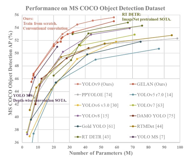
Performance of YOLOv9 on MS COCO Dataset
Yolov9: Learning What You Want to Learn Using Programmable Gradient Information
The performance of YOLOv9 on the MS COCO dataset exemplifies its significant advancements in real-time object detection, setting new benchmarks across various model sizes.
The smallest of the models, v9-S, achieved 46.8% AP on the validation set of the MS COCO dataset, while the largest model, v9-E, achieved 55.6% AP. This sets a new state-of-the-art for object detection performance.
These results demonstrate the effectiveness of YOLOv9’s techniques, such as Programmable Gradient Information (PGI) and the Generalized Efficient Layer Aggregation Network (GELAN), in enhancing the model’s learning capacity and ensuring the retention of crucial information throughout the detection process.
Training YOLOv9 on Custom Dataset
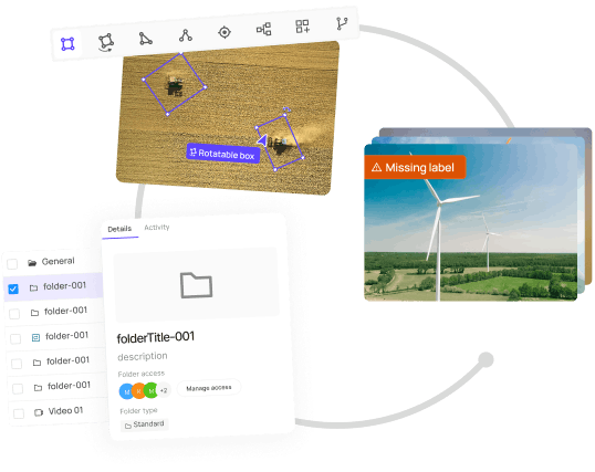
Here we will be curating a custom dataset using the Encord Index platform. Encord Index offers tools for managing and curating your data, allowing you to visualize, search, sort, and control your datasets with ease. This streamlined process ensures that your data is well-organized and ready for efficient model training and deployment.
Select New Dataset to Upload Data
You can name the dataset and add a description to provide information about the dataset.

Annotate Custom Dataset
Create an annotation project and attach the dataset and the ontology to the project to start annotation with a workflow.

You can choose manual annotation if the dataset is simple, small, and doesn’t require a review process. Automated annotation is also available and is very helpful in speeding up the annotation process.
Start Labeling
The summary page shows the progress of the annotation project. The information regarding the annotators and the performance of the annotators can be found under the tabs labels and performance.

Export the Annotation
Once the annotation has been reviewed, export the annotation in the required format.
You can use the custom dataset curated using Encord Annotate for training an object detection model. For testing YOLOv9, we are going to use an image from one of the sandbox projects on Encord Active.
Copy and run the code below to run YOLOv9 for object detection. The code for using YOLOv9 for panoptic segmentation has also been made available now on the original GitHub repository.
Installing YOLOv9
!git clone https://github.com/SkalskiP/yolov9.git
%cd yolov9
!pip install -r requirements.txt -q
!pip install -q roboflow encord av

# This is a convenience class that holds the info about Encord projects and makes everything easier.
# The class supports bounding boxes and polygons across both images, image groups, and videos.

!wget 'https://gist.githubusercontent.com/frederik-encord/e3e469d4062a24589fcab4b816b0d6ec/raw/fa0bfb0f1c47db3497d281bd90dd2b8b471230d9/encord_to_roboflow_v1.py' -O encord_to_roboflow_v1.py
Imports
from typing import Literal
from pathlib import Path

from IPython.display import Image
import roboflow

from encord import EncordUserClient
from encord_to_roboflow_v1 import ProjectConverter
Download YOLOv9 Model Weights
The YOLOv9 is available as 4 models which are ordered by parameter count:
- YOLOv9-S
- YOLOv9-M
- YOLOv9-C
- YOLOv9-E
Here we will be using gelan-c. But the same process follows for other models.
!mkdir -p {HOME}/weights!wget -q https://github.com/WongKinYiu/yolov9/releases/download/v0.1/yolov9-e-converted.pt -O {HOME}/weights/yolov9-e.pt
!wget -P {HOME}/weights -q https://github.com/WongKinYiu/yolov9/releases/download/v0.1/gelan-c.ptTrain Custom YOLOv9 Model for Object Detection
!python train.py \
--batch 8 --epochs 20 --img 640 --device 0 --min-items 0 --close-mosaic 15 \
--data $dataset_yaml_file \
--weights {HOME}/weights/gelan-c.pt \
--cfg models/detect/gelan-c.yaml \
--hyp hyp.scratch-high.yamlYOLO Object Detection using YOLOv9 on Custom Dataset
In order to perform object detection, you have to run prediction of the trained YOLOv9 on custom dataset.
Run Prediction
import torch


augment = False
visualize = False
conf_threshold = 0.25
nms_iou_thres = 0.45
max_det = 1000


seen, windows, dt = 0, [], (Profile(), Profile(), Profile())
for path, im, im0s, vid_cap, s in dataset:
    with dt[0]:
        im = torch.from_numpy(im).to(model.device).float()
        im /= 255  # 0 - 255 to 0.0 - 1.0
        if len(im.shape) == 3:
            im = im[None]  # expand for batch dim


    # Inference

 with dt[1]:
        pred = model(im, augment=augment, visualize=visualize)[0]


    # NMS
    with dt[2]:
        filtered_pred = non_max_suppression(pred, conf_threshold, nms_iou_thres, None, False, max_det=max_det)


    print(pred, filtered_pred)
    break
Generate YOLOv9 Prediction on Custom Data
import matplotlib.pyplot as plt
from matplotlib.patches import Rectangle
from PIL import Image


img = Image.open(Image path)
fig, ax = plt.subplots()
ax.imshow(img)
ax.axis("off")


for p, c in zip(filtered_pred[0], ["r", "b", "g", "cyan"]):
    x, y, w, h, score, cls = p.detach().cpu().numpy().tolist()
    ax.add_patch(Rectangle((x, y), w, h, color="r", alpha=0.2))
    ax.text(x+w/2, y+h/2, model.names[int(cls)], ha="center", va="center", color=c)


fig.savefig("/content/predictions.jpg")
YOLOv9 Vs YOLOv8: Comparative Analysis Using Encord
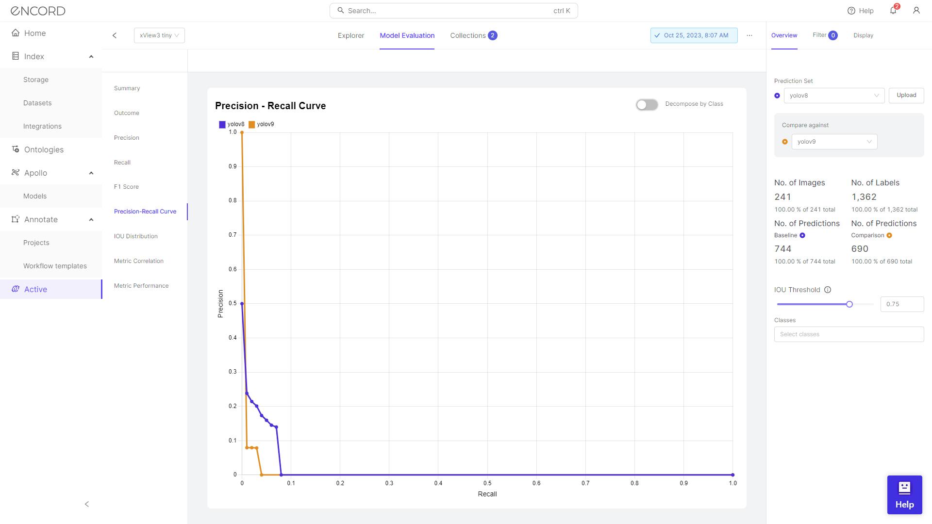
You can convert the model predictions and upload them to Encord. Here for example, the YOLOv9 and YOLOv8 have been trained and compared on the Encord platform using the xView3 dataset, which contains aerial imagery with annotations for maritime object detection.
The comparative analysis between YOLOv9 and YOLOv8 on the Encord platform focuses on precision, recall, and metric analysis. These metrics are crucial for evaluating the performance of object detection models.
- Precision: Precision measures the proportion of true positives (i.e., correct detections) among all detections. A higher precision indicates fewer false positives.
- Recall: Recall measures the proportion of actual positives that are correctly identified. A higher recall indicates fewer false negatives.
- Metric Analysis: This involves analyzing various metrics like Average Precision (AP), Mean Average Precision (mAP), etc., which provide a comprehensive view of the model’s performance.
For example, in the precision-recall curve, it seems that YOLOv8 surpasses YOLOv9 in terms of the Area Under the Curve (AUC-PR) value. This suggests that, across various threshold values, YOLOv8 typically outperforms YOLOv9 in both precision and recall. It implies that YOLOv8 is more effective at correctly identifying true positives and reducing false positives compared to YOLOv9.
But it is important to keep in mind that these two models which are being evaluated were trained for 20 epochs and are used as an example to show how to perform evaluation of trained models on custom datasets.
YOLO Real-Time Implementation
YOLO (You Only Look Once) models are widely used in real-time object detection tasks due to their speed and accuracy. Here are some real-world applications of YOLO models:
- Healthcare: YOLO models can be used in healthcare for tasks such as identifying diseases or abnormalities in medical images.
- Agriculture: YOLO models have been used to detect and classify crops, pests, and diseases, assisting in precision agriculture techniques and automating farming processes.
- Security Surveillance: YOLO models are used in security surveillance systems for real-time object detection, tracking, and classification.
- Self-Driving Cars: In autonomous vehicles, YOLO models are used for detecting objects such as other vehicles, pedestrians, traffic signs, and signals in real-time.
- Face Detection: They have also been adapted for face detection tasks in biometrics, security, and facial recognition systems
YOLO Object Detection: Key Takeaways
In this article, we provided an overview of the evolution of YOLO, from YOLOv1 to YOLOv8, and discussed its network architecture, new features, and applications. Additionally, we provided a step-by-step guide on how to use YOLOv8 for object detection and how to create model-assisted annotations with Encord Annotate.
Interested in exploring the latest releases in AI? Read our breakdown of Meta AI's SAM 2, LLama 3.1, Anthropic's Claude 3, and Grok 1.5.
Frequently asked questions
YOLOv8 is the latest iteration of the YOLO object detection model, aimed at delivering improved accuracy and efficiency over previous versions. Key updates include a more optimized network architecture, a revised anchor box design, and a modified loss function for increased accuracy.
YOLOv8 has demonstrated improved accuracy compared to earlier versions of YOLO and is competitive with state-of-the-art object detection models.
YOLOv8 is designed to run efficiently on standard hardware, making it a viable solution for real-time object detection tasks, also on edge.
There are many resources available for learning about YOLOv8, including research papers, online tutorials, and educational courses. I would recommend checking out youtube!
To use YOLOv8, you will need a computer with a GPU, deep learning framework support (such as PyTorch or TensorFlow), and access to the YOLOv8 GitHub.
Yes, the YOLOv8 codebase is open source and available for research and development purposes on GitHub here.
Yes, YOLOv8 can be fine-tuned on custom datasets to increase its accuracy for specific object detection tasks.
Anchor boxes are used in YOLOv8 to match predicted bounding boxes to ground-truth bounding boxes, improving the overall accuracy of the object detection process.
YOLOv8 is the latest iteration of the YOLO object detection model, aimed at delivering improved accuracy and efficiency over previous versions. Key updates include a more optimized network architecture, a revised anchor box design, and a modified loss function for increased accuracy.
YOLOv8 has demonstrated improved accuracy compared to earlier versions of YOLO and is competitive with state-of-the-art object detection models
YOLOv8 is designed to run efficiently on standard hardware, making it a viable solution for real-time object detection tasks, also on edge.
Anchor boxes are used in YOLOv8 to match predicted bounding boxes to ground-truth bounding boxes, improving the overall accuracy of the object detection process.
Yes, YOLOv8 can be fine-tuned on custom datasets to increase its accuracy for specific object detection tasks.
Yes, the YOLOv8 codebase is open source and available for research and development purposes on GitHub here.
To use YOLOv8, you will need a computer with a GPU, deep learning framework support (such as PyTorch or TensorFlow), and access to the YOLOv8 GitHub.
There are many resources available for learning about YOLOv8, including research papers, online tutorials, and educational courses. I would recommend checking out youtube!
YOLO requires a single forward pass through the network for predictions, making it computationally efficient.
YOLO balances performance and accuracy by processing the entire image in a single pass, making it faster and more efficient.
YOLO can detect objects in poor visibility or lighting conditions by incorporating specific modules to address these issues.
YOLOv9 can be adapted for different datasets by preparing a dataset specific to the detection task and configuring the model parameters.
YOLO stands out for its remarkable balance of speed and accuracy, enabling rapid and reliable identification of objects.
YOLOv9 has fewer parameters and requires fewer calculations, making it computationally efficient.
Fine-tuning YOLO v9 involves preparing a dataset specific to the detection task and configuring the model parameters.
YOLO handles overlapping objects by applying non-maximum suppression to eliminate duplicate or overlapping predictions.
Scaling challenges for YOLO in large-scale applications include handling varied sized multiple objects and processing of low-resolution visual contents.
Encord is designed to enhance the accuracy of detection data by providing advanced annotation capabilities that facilitate the identification of objects in complex environments. Our platform is equipped to handle the variability and inaccuracies that can arise in real-world scenarios, ensuring that models are trained on reliable datasets.
Encord's platform includes advanced annotation tools that facilitate the precise marking of defects and features in vehicle inspection images. These tools are designed to enhance accuracy and reduce manual effort, making the annotation process faster and more efficient.
Encord enables teams to build, iterate, and deploy their own object detection models with ease. The platform facilitates the annotation of various objects, such as people and vehicles, which is essential for training accurate models in real-world applications.
Encord offers specialized annotation tools for 3D object detection that streamline the labeling process for complex datasets. These tools enhance accuracy and efficiency, making it easier for teams to prepare data for training advanced machine learning models.
The Encord SDK provides robust tools for integrating custom object detection models into the platform. This integration allows teams to leverage their existing models and enhance their functionality within the Encord framework, ensuring a seamless workflow.
Encord offers various annotation primitives including bounding boxes and segmentation. Users can easily create annotations for specific objects, such as pigs, and can classify them based on behaviors or physical characteristics using the ontology builder.
Encord offers features for bounding box annotation, including the ability to toggle between different classes using hotkeys. Users can generate bounding boxes by prompting regions within the video or images, facilitating efficient object detection.
Encord supports exporting labels in common formats such as JSON for COCO panoptic and PLEX files for YOLO models. This flexibility allows users to easily switch between different annotation formats based on their project needs.
Encord supports complex pattern detection and logo detection through advanced models like YOLOv5. This integration streamlines the annotation process, making it more efficient for users working with diverse datasets.
Yes, Encord supports a variety of annotation types including bounding box and point annotations, making it suitable for diverse use cases in object detection and related tasks.