Calibration Curve

A calibration curve is a useful tool in machine learning and predictive modeling that helps  you understand and fine-tune the reliability of predicted probabilities from classification models. Having a well-calibrated model is essential for making informed decisions based on these probabilities. 

Let's take a closer look at the calibration curve, exploring its construction, interpretation, significance, and applications.

Construction of Calibration Curve

The process of constructing a calibration curve involves several key steps:

• Probabilistic Predictions: Start with a classification model that provides predicted probabilities for each instance. These predicted probabilities represent the model's confidence that an instance belongs to a certain class.
• Binning: Group instances into bins or intervals based on their predicted probabilities. Each bin contains a subset of instances that share similar predicted probabilities.
• Calculation: For each bin, calculate the average predicted probability across the instances within the bin. Simultaneously, compute the observed frequency of positive outcomes within the bin.
• Plotting: Plot the average predicted probabilities on the x-axis and the observed frequencies (or emperical probabilities) on the y-axis. The resulting plot is the calibration curve.
  

The following code provides a hands-on example of generating and plotting a calibration curve for a logistic regression model. You can adapt this code to your specific classification model and dataset, making it a valuable tool for assessing the calibration of your model's predicted probabilities.

import numpy as np
import matplotlib.pyplot as plt
from sklearn.datasets import make_classification
from sklearn.model_selection import train_test_split
from sklearn.calibration import calibration_curve
from sklearn.linear_model import LogisticRegression

# Create a synthetic dataset
X, y = make_classification(n_samples=1000, n_features=20, random_state=42)
# Split the dataset into training and testing sets
X_train, X_test, y_train, y_test = train_test_split(X, y, test_size=0.2, random_state=42)

# Train a logistic regression model
model = LogisticRegression()
model.fit(X_train, y_train)

# Predict probabilities on the test set
probabilities = model.predict_proba(X_test)[:, 1]

# Compute calibration curve
prob_true, prob_pred = calibration_curve(y_test, probabilities, n_bins=10)

# Plot the calibration curve
plt.figure(figsize=(8, 6))
plt.plot(prob_pred, prob_true, marker='o', label='Calibration Curve', color='blue')
plt.plot([0, 1], [0, 1], linestyle='--', color='gray', label='Ideal Calibration')
plt.xlabel('Mean Predicted Probability')
plt.ylabel('Fraction of Positives')
plt.title('Calibration Curve')
plt.legend()
plt.grid(True)
plt.show()

Output:

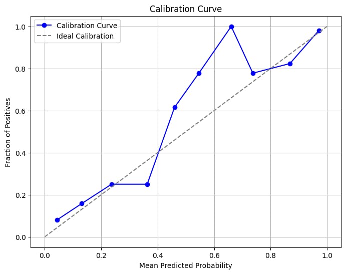
Interpretation of Calibration Curve

A perfectly calibrated model would have a calibration curve closely aligned with the 45-degree diagonal line on the plot. This line represents ideal calibration, where the predicted probabilities match the observed frequencies. Deviations from this diagonal line indicate either overconfidence or underconfidence in the model's predictions.

• Overconfidence: If the curve lies above the diagonal line, the model is overconfident. This means there are more instances with predicted probabilities close to 1 than there should be, and the model's confidence in its predictions is higher than the actual success rate.
• Underconfidence: If the curve lies below the diagonal line, the model is underconfident. In this case, instances with high predicted probabilities are less frequent than they should be and the model's confidence is lower than the actual success rate.

Significance of Calibration Curve

The calibration curve ensures that the predicted probabilities from classification models align accurately with real-world outcomes, enabling reliable interpretation and confident decision-making. By assessing the calibration curve, you can avoid overconfident or underconfident predictions, enhancing the practical utility of models.

• Reliable Probability Estimates: Predicted probabilities from a well-calibrated model can be interpreted as reliable confidence estimates. This is essential for making informed decisions based on model outputs.
• Avoiding Miscalibration: Poorly calibrated models may lead to misguided decisions. For instance, a medical diagnostic model with poor calibration might lead to inappropriate treatments.
• Robust Decision Making: Decision thresholds based on poorly calibrated models might result in suboptimal outcomes. Calibration ensures that decisions reflect the true probabilities of success.

Applications of Calibration Curve

Calibration curves have applications across various domains where accurate probability estimates are crucial for decision-making. Calibration curves are used in  healthcare diagnostics to ensure reliable medical predictions, financial credit scoring to enhance risk assessment, and fraud detection to optimize transaction security. Calibration curves play a pivotal role in delivering dependable confidence estimates that drive informed actions. 

• Medical Diagnostics: In healthcare, calibration curves help ensure that diagnostic models provide accurate and reliable confidence estimates for medical conditions.
• Credit Scoring: In finance, calibrated credit risk models provide accurate probability estimates for loan default, aiding in risk assessment.
• Fraud Detection: In fraud detection, well-calibrated models offer reliable probabilities for identifying fraudulent transactions.