Top 12 Dimensionality Reduction Techniques for Machine Learning

Dimensionality reduction is a fundamental technique in machine learning (ML) that simplifies datasets by reducing the number of input variables or features. This simplification is crucial for enhancing computational efficiency and model performance, especially as datasets grow in size and complexity.

High-dimensional datasets, often comprising hundreds or thousands of features, introduce the "curse of dimensionality." This effect slows down algorithms by making data scarceness (sparsity) and computing needs grow exponentially. 

This strategy is increasingly indispensable in the era of big data, where managing vast volumes of information is a common challenge. This article provides insight into various approaches, from classical methods like principal component analysis (PCA) and linear discriminant analysis (LDA) to advanced techniques such as manifold learning and autoencoders. 

Each technique has benefits and works best with certain data types and ML problems. This shows how flexible and different dimensionality reduction methods are for getting accurate and efficient model performance when dealing with high-dimensional data.

Here are the Twelve (12) techniques you will learn in this article:

1. Manifold Learning (t-SNE, UMAP)
2. Principal Component Analysis (PCA)
3. Independent Component Analysis (ICA)
4. Sequential Non-negative Matrix Factorization (NMF)
5. Linear Discriminant Analysis (LDA)
6. Generalized Discriminant Analysis (GDA)
7. Missing Values Ratio (MVR): Threshold Setting
8. Low Variance Filter
9. High Correlation Filter
10. Forward Feature Construction
11. Backward Feature Elimination
12. Autoencoders

Classification of Dimensionality Reduction Techniques

Dimensionality reduction techniques preserve important data, make it easier to use in other situations, and speed up learning. They do this using two steps: feature selection, which preserves the most important variables, and feature projection, which creates new variables by combining the original ones in a big way.

Feature Selection Techniques

Techniques classified under this category can identify and retain the most relevant features for model training. This approach helps reduce complexity and improve interpretability without significantly compromising accuracy. They are divided into:

• Embedded Methods: These integrate feature selection within model training, such as LASSO (L1) regularization, which reduces feature count by applying penalties to model parameters and feature importance scores from Random Forests.
• Filters: These use statistical measures to select features independently of machine learning models, including low-variance filters and correlation-based selection methods. More sophisticated filters involve Pearson’s correlation and Chi-Squared tests to assess the relationship between each feature and the target variable.
• Wrappers: These assess different feature subsets to find the most effective combination, though they are computationally more demanding.

Feature Projection Techniques

Feature projection transforms the data into a lower-dimensional space, maintaining its essential structures while reducing complexity. Key methods include:

• Manifold Learning (t-SNE, UMAP).
• Principal Component Analysis (PCA).
• Kernel PCA (K-PCA).
• Linear Discriminant Analysis (LDA).
• Quadratic Discriminant Analysis (QDA).
• Generalized Discriminant Analysis (GDA).

1. Manifold Learning

Manifold learning, a subset of non-linear dimensionality reduction techniques, is designed to uncover the intricate structure of high-dimensional data by projecting it into a lower-dimensional space.

Understanding Manifold Learning

At the heart of Manifold Learning is that while data may exist in a high-dimensional space, the intrinsic dimensionality—representing the true degrees of freedom within the data—is often much lower.

Core Techniques and Algorithms

1. t-Distributed Stochastic Neighbor Embedding (t-SNE): t-SNE is powerful for visualizing high-dimensional data in two or three dimensions. It converts similarities between data points to joint probabilities and minimizes the divergence between them in different spaces, excelling in revealing clusters within data.
2. Uniform Manifold Approximation and Projection (UMAP): UMAP is a relatively recent technique that balances the preservation of local and global data structures for superior speed and scalability. It's computationally efficient and has gained popularity for its ability to handle large datasets and complex topologies.
3. Isomap (Isometric Mapping): Isomap extends classical Multidimensional Scaling (MDS) by incorporating geodesic distances among points. It's particularly effective for datasets where the manifold (geometric surface) is roughly isometric to a Euclidean space, allowing global properties to be preserved.
4. Locally Linear Embedding (LLE): LLE reconstructs high-dimensional data points from their nearest neighbors, assuming the manifold is locally linear. By preserving local relationships, LLE can unfold twisted or folded manifolds.

2. Principal Component Analysis (PCA)

The Principal Component Analysis (PCA) algorithm is a method used to reduce the dimensionality of a dataset while preserving as much information (variance) as possible. As a linear reduction method, PCA transforms a complex dataset with many variables into a simpler one that retains critical trends and patterns.

What is Principal Component Analysis (PCA)?

PCA identifies and uses the principal components (directions that maximize variance and are orthogonal to each other) to effectively project data into a lower-dimensional space. This process begins with standardizing the original variables, ensuring their equal contribution to the analysis by normalizing them to have a zero mean and unit variance.

Step-by-Step Explanation of Principal Component Analysis

1. Standardization: Normalize the data so each variable contributes equally, addressing PCA's sensitivity to variable scales.
2. Covariance Matrix Computation: Compute the covariance matrix to understand how the variables of the input dataset deviate from the mean and to see if they are related (i.e., correlated).
3. Finding Eigenvectors and Eigenvalues: Find the new axes (eigenvectors) that maximize variance (measured by eigenvalues), making sure they are orthogonal to show that variance can go in different directions.
4. Sorting and Ranking: Prioritize eigenvectors (and thus principal components) by their ability to capture data variance, using eigenvalues as the metric of importance.
5. Feature Vector Formation: Select a subset of eigenvectors based on their ranking to form a feature vector. This subset of eigenvectors forms the principal components.
6. Transformation: Map the original data into this principal component space, enabling analysis or further machine learning in a more tractable, less noisy space.

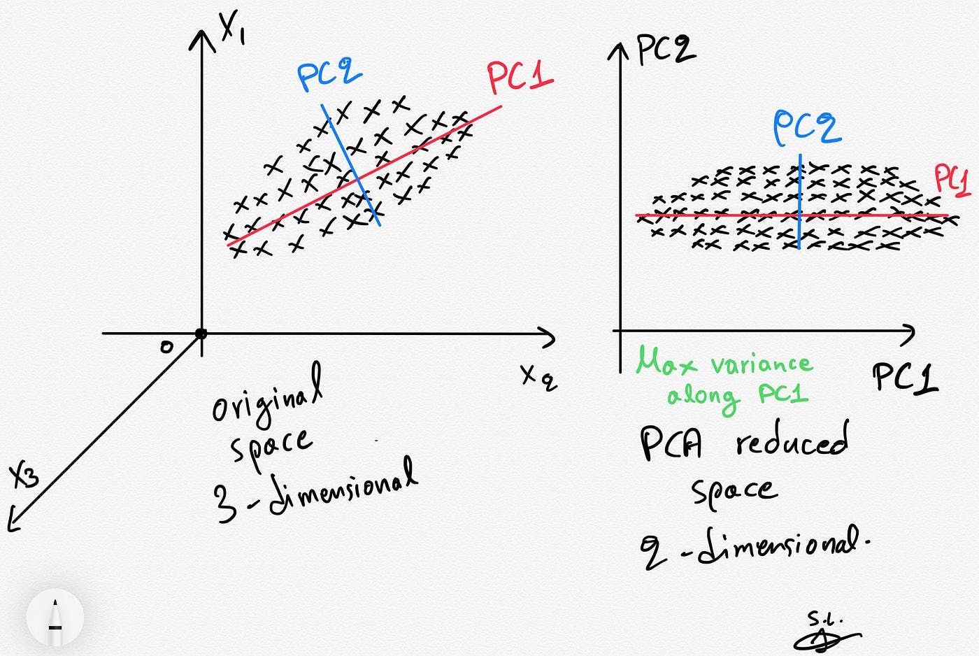
Dimensionality reduction using PCA

Applications

PCA is widely used in exploratory data analysis and predictive modeling. It is also applied in areas like image compression, genomics for pattern recognition, and financial data for uncovering latent patterns and correlations. 

PCA can help visualize complex datasets by reducing data dimensionality. It can also make machine learning algorithms more efficient by reducing computational costs and avoiding overfitting with high-dimensional data.

3. Independent Component Analysis (ICA)

Independent Component Analysis (ICA) is a computational method in signal processing that separates a multivariate signal into additive, statistically independent subcomponents. Statistical independence is critical because Gaussian variables maximize entropy given a fixed variance, making non-Gaussianity a key indicator of independence. 

Originating from the work of Hérault and Jutten in 1985, ICA excels in applications like the "cocktail party problem," where it isolates distinct audio streams amid noise without prior source information.

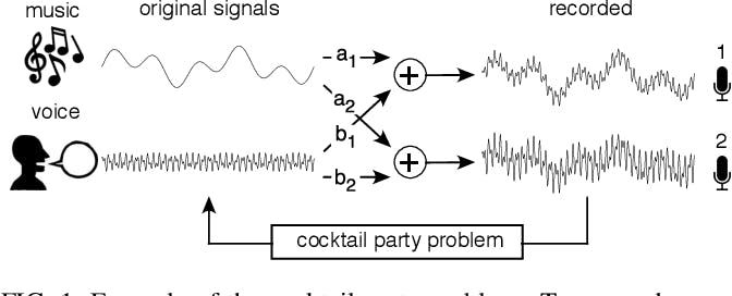
Example of the cocktail party problem

The cocktail party problem involves separating original sounds, such as music and voice, from mixed signals recorded by two microphones. Each microphone captures a different combination of these sounds due to its varying proximity to the sound sources.

Principles Behind Independent Component Analysis

The essence of ICA is its focus on identifying and separating independent non-Gaussian signals embedded within a dataset. It uses the fact that these signals are statistically independent and non-Gaussian to divide the mixed signals into separate parts from different sources. 

This demixing process is pivotal, transforming seemingly inextricable data (impossible to separate) into interpretable components.

Algorithmic Process

To achieve its goals, ICA incorporates several preprocessing steps:

• Centering adjusts the data to have a zero mean, ensuring that analyses focus on variance rather than mean differences.
• Whitening transforms the data into uncorrelated variables, simplifying the subsequent separation process.
• After these steps, ICA applies iterative methods to separate independent components, and it often uses auxiliary methods like PCA or singular value decomposition (SVD) to lower the number of dimensions at the start. This sets the stage for efficient and robust component extraction.

By breaking signals down into basic, understandable parts, ICA provides valuable information and makes advanced data analysis easier, which shows its importance in modern signal processing and beyond. Let’s see some of its applications.

Applications of ICA

The versatility of ICA is evident across various domains:

• In telecommunications, it enhances signal clarity amidst interference.
• Finance benefits from its ability to identify underlying factors in complex market data, assess risk, and detect anomalies.
• In biomedical signal analysis, it dissects EEG or fMRI data to isolate neurological activity from artifacts (such as eye blinks).

Collaborative DICOM annotation platform for medical imaging

CT, X-ray, mammography, MRI, PET scans, ultrasound

See it in action

4. Sequential Non-negative Matrix Factorization (NMF)

Nonnegative matrix Factorization (NMF) is a technique in multivariate analysis and linear algebra in which a matrix V is factorized into two lower-dimensional matrices, W (basis matrix) and H (coefficient matrix), with the constraint that all matrices involved have no negative elements. 

This factorization works especially well for fields where the data is naturally non-negative, like genetic expression data or audio spectrograms, because it makes it easy to understand the parts. 

Principle of Sequential Non-negative Matrix Factorization

The distinctive aspect of Sequential NMF is its iterative approach to decomposing matrix V into  W and H, making it adept at handling time-series data or datasets where the temporal evolution of components is crucial.

This is particularly relevant in dynamic datasets or applications where data evolves. Sequential NMF responds to changes by repeatedly updating W and H, capturing changing patterns or features important in online learning, streaming data, or time-series analysis.

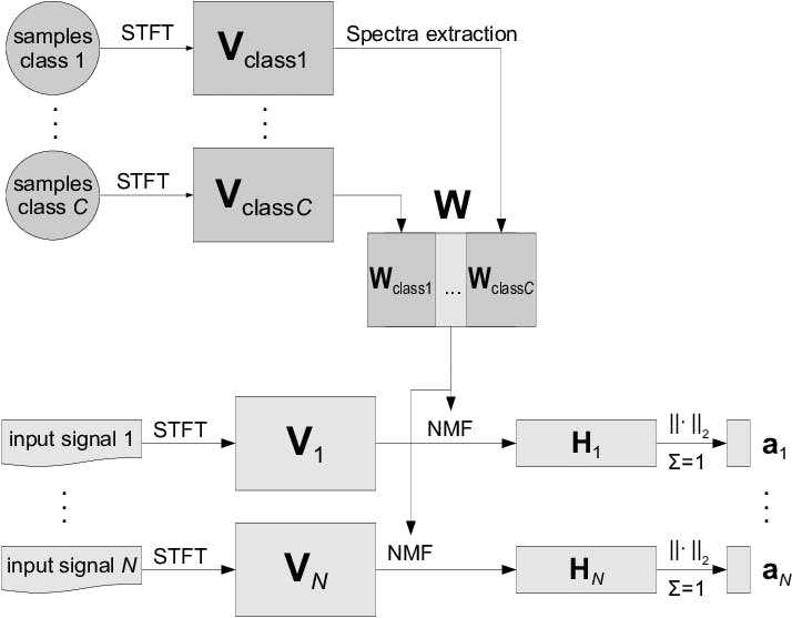
Procedure of feature extraction using NMF

Applications

The adaptability of Sequential NMF has led to its application in a broad range of fields, including:

• Medical Research: In oncology, Sequential NMF plays a pivotal role in analyzing genetic data over time, aiding in the classification of cancer types, and identifying temporal patterns in biomarker expression.
• Audio Signal Processing: It is used to analyze sequences of audio signals and capture the temporal evolution of musical notes or speech.
• Astronomy and Computer Vision: Sequential NMF tracks and analyzes the temporal changes in celestial bodies or dynamic scenes.
  

5. Linear Discriminant Analysis (LDA)

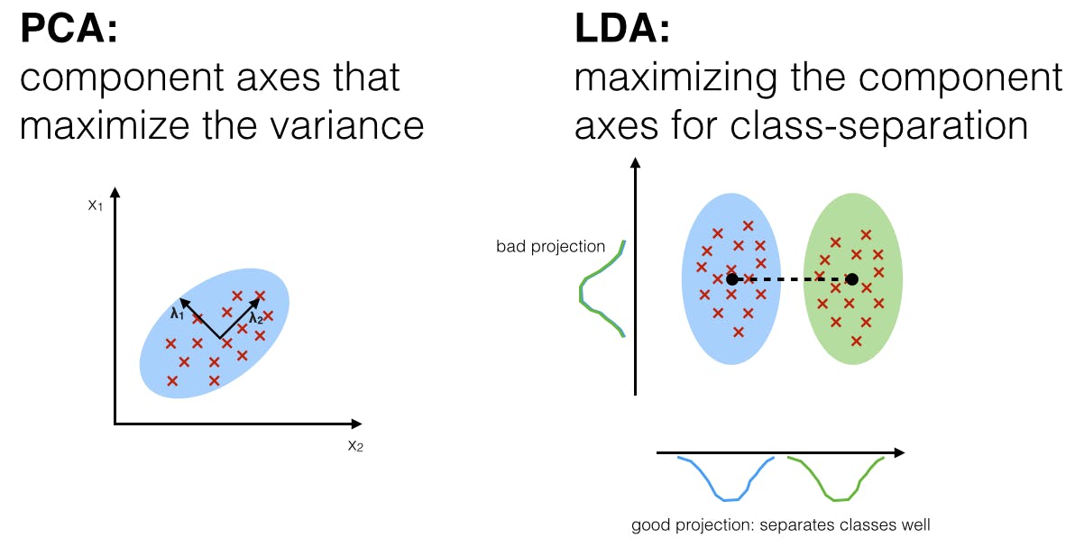
Linear Discriminant Analysis (LDA) is a supervised machine learning technique used primarily for pattern classification, dimensionality reduction, and feature extraction. It focuses on maximizing class separability. 

Unlike PCA, which optimizes for variance regardless of class labels, LDA aims to find a linear combination of features that separates different classes. It projects data onto a lower-dimensional space using class labels to accomplish this.

This method is highly efficient in scenarios where the division between categories of data is to be accentuated.

PCA Vs. LDA: What's the Difference?

Assumptions of LDA

Linear Discriminant Analysis (LDA) operates under assumptions essential for effectively classifying observations into predefined groups based on predictor variables. These assumptions, elaborated below, play a critical role in the accuracy and reliability of LDA's predictions.

1. Multivariate Normality: Each class must follow a multivariate normal distribution (multi-dimensional bell curve). You can asses this through visual plots or statistical tests before applying LDA.
2. Homogeneity of Variances (Homoscedasticity): Ensuring uniform variance across groups helps maintain the reliability of LDA's projections. Techniques like Levene's test can assess this assumption.
3. Absence of Multicollinearity: LDA requires predictors to be relatively independent. Techniques like variance inflation factors (VIFs) can diagnose multicollinearity issues.

Working Methodology of Linear Discriminant Analysis 

LDA transforms the feature space into a lower-dimensional one that maximizes class separability by:

1. Calculating mean vectors for each class.
2. Computing within-class and between-class scatter matrices to understand the distribution and separation of classes.
3. Solving for the eigenvalues and eigenvectors that maximize the between-class variance relative to the within-class variance. This defines the optimal projection space to distinguish the classes.

Tools like Python's Scikit-learn library simplify applying LDA with functions specifically designed to carry out these steps efficiently.

Applications

LDA's ability to reduce dimensionality while preserving as much of the class discriminatory information as possible makes it a powerful feature extraction and classification tool applicable across various domains. Examples:

• In facial recognition, LDA enhances the distinction between individual faces to improve recognition accuracy.
• Medical diagnostics benefit from LDA's ability to classify patient data into distinct disease categories, aiding in early and accurate diagnosis.
• In marketing, LDA helps segment customers for targeted marketing campaigns based on demographic and behavioral data.

6. Generalized Discriminant Analysis (GDA)

Generalized Discriminant Analysis (GDA) extends linear discriminant analysis (LDA) into a nonlinear domain. It uses kernel functions to project input data vectors into a higher-dimensional feature space to capture complex patterns that LDA, limited to linear boundaries, might miss. 

These functions project data into a higher-dimensional space where inseparable classes in the original space can be distinctly separated.

Step-by-step Explanation of Generalized Discriminant Analysis 

The core objective of GDA is to find a low-dimensional projection that maximizes the between-class scatter while minimizing the within-class scatter in the high-dimensional feature space.

Let’s examine the GDA algorithm step by step:

1. Kernel Function Selection: First, choose an appropriate kernel function (e.g., polynomial, radial basis function (RBF)) that transforms the input data into a higher-dimensional space.

2. Kernel Matrix Computation: Compute the kernel matrix K, representing the high-dimensional dot products between all pairs of data points. This matrix is central to transforming the data into a feature space without explicitly performing the computationally expensive mapping.

3. Scatter Matrix Calculation in Feature Space: In the feature space, compute the within-class scatter matrix SW and the between-class scatter matrix SB, using the kernel matrix K to account for the data's nonlinear transformation.

4. Eigenvalue Problem: Solving this problem in the feature space identifies the projection vectors that best separate the classes by maximizing the SB/SW ratio. This step is crucial for identifying the most informative projections for class separation.

5. Projection: Use the obtained eigenvectors to project the input data onto a lower-dimensional space that maximizes class separability to achieve GDA's goal of improved class recognition.

Applications

GDA has been applied in various domains, benefiting from its ability to handle nonlinear patterns:

• Image and Video Recognition: GDA is used for facial recognition, object detection, and activity recognition in videos, where the data often exhibit complex, nonlinear relationships.
• Biomedical Signal Processing: In analyzing EEG, ECG signals, and other biomedical data, GDA helps distinguish between different physiological states or diagnose diseases.
• Text Classification and Sentiment Analysis: GDA transforms text data into a higher-dimensional space, effectively separating documents or sentiments that are not linearly separable in the original feature space.

7. Missing Values Ratio (MVR): Threshold Setting

Datasets often contain missing values, which can significantly impact the effectiveness of dimensionality reduction techniques. One approach to addressing this challenge is to utilize a missing values ratio (MVR) thresholding technique for feature selection.

Process of Setting Threshold for Missing Values 

The MVR for a feature is calculated as the percentage of missing values for data points. The optimal threshold is dependent on several factors, including the dataset’s nature and the intended analysis:

1. Determining the Threshold: Use statistical analyses, domain expertise, and exploratory data analysis (e.g., histograms of missing value ratios) to identify a suitable threshold. This decision balances retaining valuable data against excluding features that could introduce bias or noise.
2. Implications of Threshold Settings: A high threshold may retain too many features with missing data, complicating the analysis. Conversely, a low threshold could lead to excessive data loss. Regularly, thresholds between 20% to 60% are considered, but this range varies widely based on the data context and analysis goals.
3. Contextual Considerations: The dataset's specific characteristics and the chosen dimensionality reduction technique influence the threshold setting. Methods sensitive to data sparsity or noise may require a lower MVR threshold.

Applications

• High-throughput Biological Data Analysis: Technical limitations often render Gene expression data incomplete. Setting a conservative MVR threshold may preserve crucial biological insights by retaining genes with marginally incomplete data.
• Customer Data Analysis: Customer surveys may have varying completion rates across questions. MVR thresholding identifies which survey items provide the most complete and reliable data, sharpening customer insights.
• Social Media Analysis: Social media data can be sparse, with certain users' entries missing. MVR thresholding can help select informative features for user profiling or sentiment analysis.
  

8. Low Variance Filter

A low variance filter is a straightforward preprocessing technique aimed at reducing dimensionality by eliminating features with minimal variance, focusing analysis on more informative aspects of the dataset.

Steps for Implementing a Low Variance Filter

1. Calculate Variance: For each feature in the dataset, compute the variance. Prioritize scaling or normalizing data to ensure variance is measured on a comparable basis across all features.
2. Set Threshold: Define a threshold for the minimum acceptable variance. This threshold often depends on the specific dataset and analysis objectives but typically ranges from a small percentage of the total variance observed across features.
3. Feature Selection: Exclude features with variances below the threshold. Tools like Python's `pandas` library or R's `caret` package can efficiently automate this process.

Applications of Low Variance Filter Across Domains

• Sensor Data Analysis: Sensor readings might exhibit minimal fluctuation over time, leading to features with low variance. Removing these features can help focus on the sensor data's more dynamic aspects.
• Image Processing: Images can contain features representing background noise. These features often have low variance and can be eliminated using the low variance filter before image analysis.
• Text Classification: Text data might contain stop words or punctuation marks that offer minimal information for classification. The low variance filter can help remove such features, improving classification accuracy.

9. High Correlation Filter

The high correlation filter is a crucial technique for addressing feature redundancy. Eliminating highly correlated features optimizes datasets for improved model accuracy and efficiency.

Steps for Implementing a High Correlation Filter

1. Compute Correlation Matrix: Assess the relationship between all feature pairs using an appropriate correlation coefficient, such as Pearson for continuous features (linear relationships) and Spearman for ordinal (monotonic relationships).
2. Define Threshold: Establish a correlation coefficient threshold above highly correlated features. A common threshold of 0.8 or 0.9 may vary based on specific model requirements and data sensitivity.
3. Feature Selection: Identify sets of features whose correlation exceeds the threshold. From each set, retain only one feature based on criteria like predictive power, data completeness, or domain relevance and remove the others.

Applications

• Financial Data Analysis: Stock prices or other financial metrics might exhibit a high correlation, often reflecting market trends. The high correlation filter can help select a representative subset of features for financial modeling.
• Bioinformatics: Gene expression data can involve genes with similar functions, leading to high correlation. Selecting a subset of uncorrelated genes can be beneficial for identifying distinct biological processes.
• Recommendation Systems: User profiles often contain correlated features like similar purchase history or browsing behavior. The high correlation filter can help select representative features to build more efficient recommendation models.

10. Forward Feature Construction

Forward Feature Construction (FFC) is a methodical approach to feature selection, designed to incrementally build a model by adding features that offer the most significant improvement. This technique is particularly effective when the relationship between features and the target variable is complex and needs to be fully understood.

Algorithm for Forward Feature Construction

1. Initiate with a Null Model: Start with a baseline model without any predictors to establish a performance benchmark.
2. Evaluation Potential Additions: For each candidate feature outside the model, assess potential performance improvements by adding that feature. 
3. Select the Best Feature: Incorporate the feature that significantly improves performance. Ensure the model remains interpretable and manageable.
4. Iteration: Continue adding features until further additions fail to offer significant gains, considering computational efficiency and the risk of diminishing returns.

Practical Considerations and Implementation

• Performance Metrics: To gauge improvements, use appropriate metrics, such as the Akaike Information Criterion (AIC) for regression or accuracy and the F1 score for classification, adapting the choice of metric to the model's context.
• Challenges: Be mindful of computational demands and the potential for multicollinearity. Implementing strategies to mitigate these risks, such as pre-screening features or setting a cap on the number of features, can be crucial.
• Tools: Leverage software tools and libraries (e.g., R's `stepAIC` or Python's `mlxtend.SequentialFeatureSelector`) that support efficient FFC application and streamline feature selection.

Applications of FFC Across Domains

• Clinical Trials Prediction: In clinical research, FFC facilitates the identification of the most predictive biomarkers or clinical variables from a vast dataset, optimizing models for outcome prediction.
• Financial Modeling:  In financial market analysis, this method distills a complex set of economic indicators down to a core subset that most accurately forecasts market movements or financial risk.

11. Backward Feature Elimination

Backward Feature Elimination (BFE) systematically simplifies machine learning models by iteratively removing the least critical features, starting with a model that includes the entire set of features. This technique is particularly suited for refining linear and logistic regression models, where dimensionality reduction can significantly improve performance and interpretability.

Algorithm for Backward Feature Elimination

1. Initialize with Full Model: Construct a model incorporating all available features to establish a comprehensive baseline.
2. Identify and Remove Least Impactful Feature: Determine the feature whose removal least affects or improves the model's predictive performance. Use metrics like p-values or importance scores to eliminate it from the model.
3. Performance Evaluation: After each removal, assess the model to ensure performance remains robust. Utilize cross-validation or similar methods to validate performance objectively.
4. Iterative Optimization: Continue this evaluation and elimination process until further removals degrade model performance, indicating that an optimal feature subset has been reached.

Practical Considerations for Implementation

• Computational Efficiency: Given the potentially high computational load, especially with large feature sets, employ strategies like parallel processing or stepwise evaluation to simplify the Backward Feature Elimination (BFE) process.
• Complex Feature Interactions: Special attention is needed when features interact or are categorical. Consider their relationships to avoid inadvertently removing significant predictors.

Applications

Backward Feature Elimination is particularly useful in contexts like:

• Genomics: In genomics research, BFE helps distill large datasets into a manageable number of significant genes to improve understanding of genetic influences on diseases.
• High-dimensional Data Analysis: BFE simplifies complex models in various fields, from finance to the social sciences, by identifying and eliminating redundant features. This could reduce overfitting and improve the model's generalizability.

12. Autoencoders

Autoencoders are a unique type of neural network used in deep learning, primarily for dimensionality reduction and feature learning. They are designed to encode inputs into a compressed, lower-dimensional form and reconstruct the output as closely as possible to the original input.

This process emphasizes the encoder-decoder structure. The encoder reduces the dimensionality, and the decoder attempts to reconstruct the input from this reduced encoding.

How Does Autoencoders Work?

They achieve dimensionality reduction and feature learning by mimicking the input data through encoding and decoding.

1. Encoding: Imagine a bottle with a narrow neck in the middle. The data (e.g., an image) is the input that goes into the wide top part of the bottle. The encoder acts like this narrow neck, compressing the data into a smaller representation. This compressed version, often called the latent space representation, captures the essential features of the original data.

• The encoder is typically made up of multiple neural network layers that gradually reduce the dimensionality of the data.
• The autoencoder learns to discard irrelevant information and focus on the most important characteristics by forcing the data through this bottleneck.

2. Decoding: Now, imagine flipping the bottle upside down. The decoder acts like the wide bottom part, trying to recreate the original data from the compressed representation that came through the neck.

• The decoder also uses multiple neural network layers, but this time, it gradually increases the data's dimensionality, aiming to reconstruct the original input as accurately as possible.
  

Variants and Advanced Applications

• Sparse Autoencoders: Introduce regularization terms to enforce sparsity in the latent representation, enhancing feature selection.
• Denoising Autoencoders: Specifically designed to remove noise from data, these autoencoders learn to recover clean data from noisy inputs, offering superior performance in image and signal processing tasks.
• Variational Autoencoders (VAEs): VAEs make new data samples possible by treating the latent space as a probabilistic distribution. This opens up new ways to use generative modeling.
  

Training Nuances

• Autoencoders use optimizers like Adam or stochastic gradient descent (SGD) to improve reconstruction accuracy by improving their weights through backpropagation.
• Overfitting prevention is integral and can be addressed through methods like dropout, L1/L2 regularization, or a validation set for early stopping.
  

Applications

Autoencoders have a wide range of applications, including but not limited to:

• Dimensionality Reduction: Similar to PCA but more powerful (as non-linear alternatives), autoencoders can perform non-linear dimensionality reductions, making them particularly useful for preprocessing steps in machine learning pipelines.
• Image Denoising: By learning to map noisy inputs to clean outputs, denoising autoencoders can effectively remove noise from images, surpassing traditional denoising methods in efficiency and accuracy.
• Generative modeling: Variational autoencoders (VAEs) can make new data samples similar to the original input data by modeling the latent space as a continuous probability distribution.​​ (e.g., Generative Adversarial Networks (GANs)).

Impact of Dimensionality Reduction in Smart City Solutions

Automotus is a company at the forefront of using AI to revolutionize smart city infrastructure, particularly traffic management.  They achieve this by deploying intelligent traffic monitoring systems that capture vast amounts of video data from urban environments. 

However, efficiently processing and analyzing this high-dimensional data presents a significant challenge. This is where dimensionality reduction techniques come into play.

The sheer volume of video data generated by Automotus' traffic monitoring systems necessitates dimensionality reduction techniques to make data processing and analysis manageable. 

PCA identifies the most significant features in the data (video frames in this case) and transforms them into a lower-dimensional space while retaining the maximum amount of variance. This allows Automotus to extract the essential information from the video data, such as traffic flow patterns, vehicle types, and potential congestion points, without analyzing every pixel.

Partnering with Encord, Automotus led to a 20% increase in model accuracy and a 35% reduction in dataset size. This collaboration focused on dimensionality reduction, leveraging Encord Annotate’s flexible ontology, quality control capabilities, and automated labeling features. 

That approach helped Automotus reduce infrastructure constraints, improve model performance to provide better data to clients, and reduce labeling costs. Efficiency directly contributes to Automotus's business growth and operational scalability.

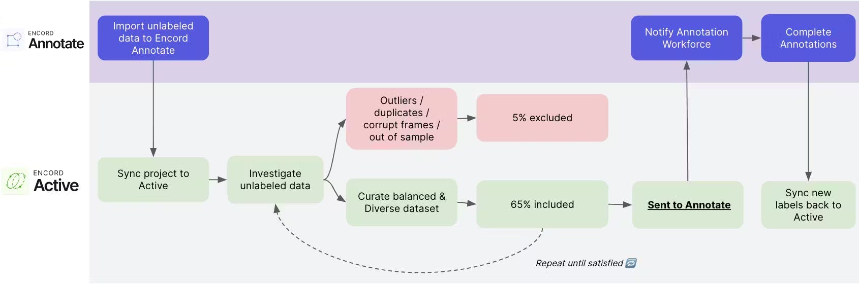
The team used Encord Active to visually inspect, query, and sort their datasets to remove unwanted and poor-quality data with just a few clicks, leading to a 35% reduction in the size of the datasets for annotation. This enabled the team to cut their labeling costs by over a third.

Dimensionality Reduction Technique: Key Takeaways

• Dimensionality reduction techniques simplify models and enhance computational efficiency.
• They help manage the "curse of dimensionality," improving model generalizability and reducing overfitting risk.
• These techniques are used for feature selection and extraction, contributing to better model performance.

They are applied in various fields, such as image and speech recognition, financial analysis, and bioinformatics, showcasing their versatility.

• By reducing the number of input variables, these methods ensure models are computationally efficient and capture essential data patterns for more accurate predictions.