Object Classification with Caltech 101

Object classification is a computer vision technique that identifies and categorizes objects within an image or video. In this article, we give you all the information you need to apply object detection to the Caltech 101 Dataset.

Object classification involves using machine learning algorithms, such as deep neural networks, to analyze the visual features of an image and then make predictions about the class or type of objects present in the image.

What is Object classification? 

Object classification is often used in applications such as self-driving cars, where the vehicle must be able to recognize and classify different types of objects on the road, such as pedestrians, traffic signs, and other vehicles. 

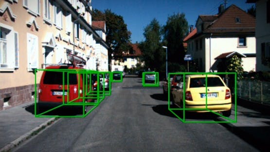
Object classification for self-driving cars

Source

It’s also used in image recognition tasks, such as identifying specific objects within an image or detecting anomalies or defects in manufacturing processes.

Object classification algorithms typically involve several steps, including feature extraction and classification. In the feature extraction step, the algorithm identifies visual features such as edges, shapes, and patterns that are characteristic of the objects in the image. These features are then used to classify the objects into predefined classes or categories, such as "car", "dog", "person", etc.

The classification step involves using machine learning algorithms, such as deep neural networks, to analyze the visual features of an image and predict the class or type of object present in the image. The model is trained on a large dataset of labeled images, where the algorithm weights are adjusted iteratively to minimize the error between the predicted and actual labels.

Once trained, a computer vision (CV) or machine learning (ML) model can be used to classify objects in new images by analyzing their visual features and predicting the class of the object.

Object classification is a challenging task due to the variability in object appearance caused by factors such as lighting, occlusion, and pose. However, advances in machine learning and computer vision techniques have significantly improved object classification accuracy in recent years, making it an increasingly important technology in many fields.

Importance of Object Classification in Computer Vision

Here are some reasons why object classification is important in computer vision:

• Object classification enables algorithmic models to interpret and understand the visual world around them. By identifying objects within an image or video, ML models can extract meaningful information, such as object location, size, and orientation, and use this information to make informed decisions.
  
• Object classification is critical for tasks such as object tracking, object detection, and object recognition. These tasks are essential in applications such as autonomous vehicles, where machines must be able to detect and track objects such as pedestrians, other vehicles, and obstacles in real-time.
  
• Object classification is a key component of image and video search. By classifying objects within images and videos, machines can accurately categorize and index visual data, making searching and retrieving relevant content easier.
  
• Object classification is important for medical imaging, where it can be used to detect and diagnose diseases and abnormalities. For example, object classification can be used to identify cancerous cells within a medical image, enabling early diagnosis and treatment.

Overall, object classification is an important task in computer vision, which enables machines to understand and interpret the visual world around them, making it a crucial technology in a wide range of applications.

Caltech 101 Dataset

Caltech 101 is a very popular dataset for object recognition in computer vision. 

It contains images from 101 object categories like “helicopter”, “elephant”, and “chair”, etc, and background categories that contain the images not from the 101 object categories. There are about 40 to 400 images for each object category, while most classes have about 50 images.

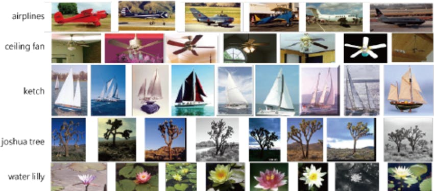
Images in the Caltech101 dataset

Object recognition algorithms can be divided into two groups: recognition of individual objects, and categories. 

The training of a machine learning model for individual object recognition is easier. But to build a lightweight, light-invariant, and viewpoint variant model, you need a diverse dataset.

Categories are more general, require more complex representations, and are more difficult to learn. The appearance of objects within a given category may be highly variable; therefore the model should be flexible enough to handle this.

Many machine learning practitioners or researchers use Caltech 101 dataset to benchmark the state-of-the-art object recognition models. 

The images in all 101 object categories are captured under varying lighting conditions, backgrounds, and viewpoints, making the dataset a good candidate for training a robust computer vision model.

Apart from being used for training object recognition algorithms, Caltech 101 is also used for various other tasks like fine-grained image classification, density estimation, semantic correspondence, unsupervised anomaly detection, and semi-supervised image classification. 

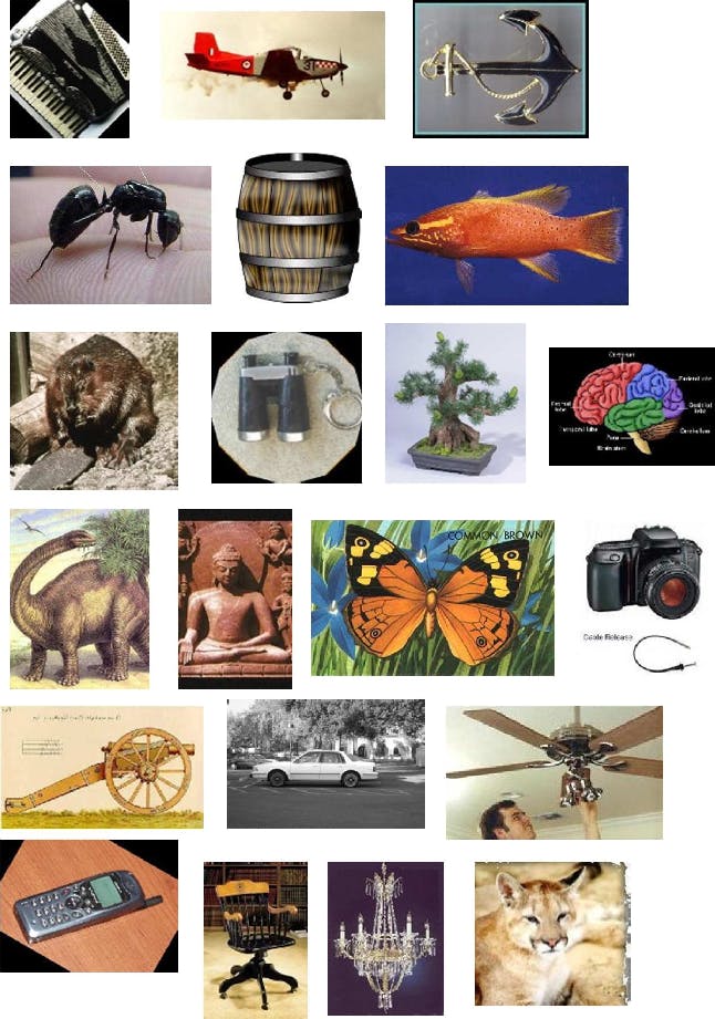
More examples of images from Caltech101

For example, Caltech 101 was used in the paper AutoAugment:Learning augmentation policies from data. This paper proposes a procedure called AutoAugment to automatically search for improved data augmentation policies. Here, they test the transferable property of the augmentation policies by transferring the policies learned on ImageNet to Caltech 101. 

About the Dataset

• Research Paper: Learning generative visual models from few training examples: An incremental Bayesian approach tested on 101 object categories
• Authors: Fei-Fei Li, Marco Andreetto, Marc ‘Aurelio Ranzato and Pietro Perona
• Dataset Size: 9146
• Categories: 101
• Resolution: ~300200 pixels
• Dataset Size: 1.2 GB
• License: Creative Common Attribution 4.0 International
• Release: September 2003
• Webpage: Caltech webpage, TensorFlow webpage, Torchvision webpage

Advantages of using Caltech 101

There are several advantages of using Caltech 101 over similar object recognition datasets, such as:

• Uniform size and presentation: Most of the images within each category are uniform in image size and in the relative position of objects of interest. 
• Low level of clutter/occlusion: Object recognition algorithms usually store features unique to the object. With a low level of clutter and occlusion, the features would be unique and transferable as well. 
• High-quality annotations: The dataset comes with high-quality annotations which are collected from real-world scenarios, making it a more realistic dataset. High-quality annotations are crucial for classification tasks as they provide the ground truth labels necessary to train and evaluate machine learning algorithms, ensuring the accuracy and reliability of the results. 

Disadvantages of the Caltech 101

There are a few trade-offs with the Caltech 101 dataset which include:

• Uniform dataset: The images in the dataset are very uniform and usually not occluded. Hence, object recognition models solely trained on this dataset might not perform well in real-world applications. 
• Limited object classes: Although the dataset contains 101 object categories, it may not be representative of all possible object categories which can limit the dataset’s applicability to real-world scenarios. For example, medical images, industrial objects like machinery, tools, or equipment, or cultural artifacts like artworks, historical objects, or cultural heritage sites. 
• Aliasing and artifacts due to manipulation: Some images have been rotated and scaled from their original orientation, and suffer from some amount of aliasing. 

However, analyzing a dataset for a computer vision model requires more detailed information about the dataset. It helps in determining if the dataset is fit for your project. With Encord Active you can easily explore the datasets/labels and its distribution. We get information about the quality of the data and labels. 

Understanding the data and label distribution, quality, and other related information can help computer vision practitioners determine if the dataset is suitable for their project and avoid potential biases or errors in their models.

How to download the Caltech 101 Dataset?

Since it’s a popular dataset, there are few dataset loaders available. 

PyTorch

If you want to use Pytorch for downloading the dataset, please follow the documentation. 

torchvison.datasets.Caltech101()

TensorFlow

If you are using TensorFlow for building your computer vision model and want to download the dataset, please follow the instructions in the link. To load the dataset as a single Tensor,

(img_train, label_train), (img_test, label_test) = tfds.as_numpy(tfds.load('caltech101', split=['train', 'test'], batch_size = -1, as_supervised=True))

And its source code is

tfds.datasets.caltech101.Builder

You can also find this here.

Encord Active

We will be downloading the dataset using Encord Active here in this blog. It is an open-source active learning toolkit that helps in visualizing the data, evaluating computer vision models, finding model failure modes, and much more. 

Run the following commands in your favorite Python environment with the following commands:

python3.9 -m venv ea-venv
source ea-venv/bin/activate
# within venv
pip install encord-active

Or you can follow through the following command to install Encord Active using GitHub:

pip install git+https://github.com/encord-team/encord-active

To check if Encord Active has been installed, run:

encord-active --help

Encord Active has many sandbox datasets like the MNIST, BDD100K, TACO datasets, and much more. The Caltech101 dataset is one of them. These sandbox datasets are commonly used in computer vision applications for building benchmark models.

Now that you have Encord Active installed, let’s download the Caltech101 dataset by running the command:

encord-active download

The script asks you to choose a project, navigate the options ↓ and ↑ select the Caltech-101 train or test dataset, and hit enter. The dataset has been pre-divided into a training set comprising 60% of the data and a testing set comprising 40% of the data for the convenience of analyzing the dataset.

Easy! Now, you got your data. In order to visualize the data in the browser, run the command:

cd /path/to/downloaded/project
encord-active visualize

The image below shows the webpage that opens in your browser showing the data and its properties. Let’s analyze the properties we can visualize here.

Visualize the data in your browser (data = Caltech-101 training data-60% of Caltech-101 dataset)

Data Quality of the Caltech 101 Dataset

We navigate to the Data Quality → Summary page to assess data quality. The summary page contains information like the total number of images, image size distribution, etc. It also gives an overview of how many issues Encord Active has detected on the dataset and tells you which metric to focus on.

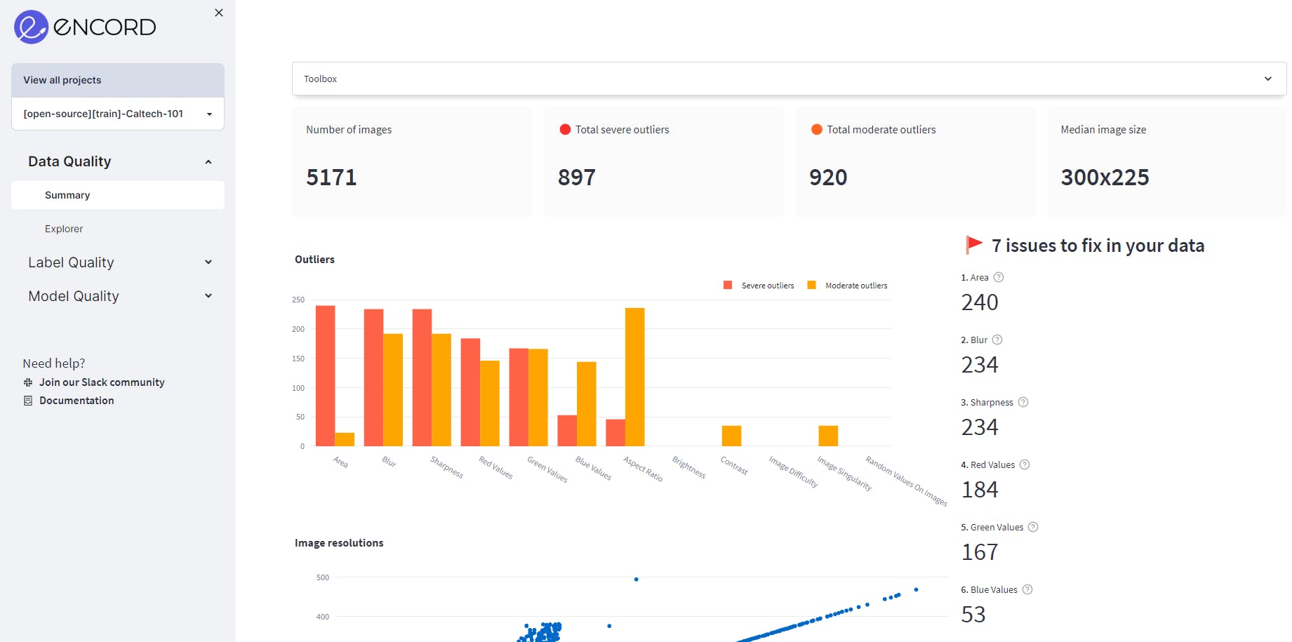
The summary tab of Data Quality

The Data Quality → Explorer page contains detailed information about different metrics and the data distribution with each metric. A few of the metrics are discussed below:

2D Embeddings

In machine learning, a 2D embedding for an image is a technique to transform high-dimensional image data into a 2D space while preserving the most important features and characteristics of the image. 

The 2D embedding plot here is a scatter plot with each point representing a data point in the dataset. The position of each point on the plot reflects the relative similarity or dissimilarity of the data points with respect to each other. For example, select the box or the Lasso Select in the upper right corner of the plot. Once you select a region, you can visualize the images only in the selected region.

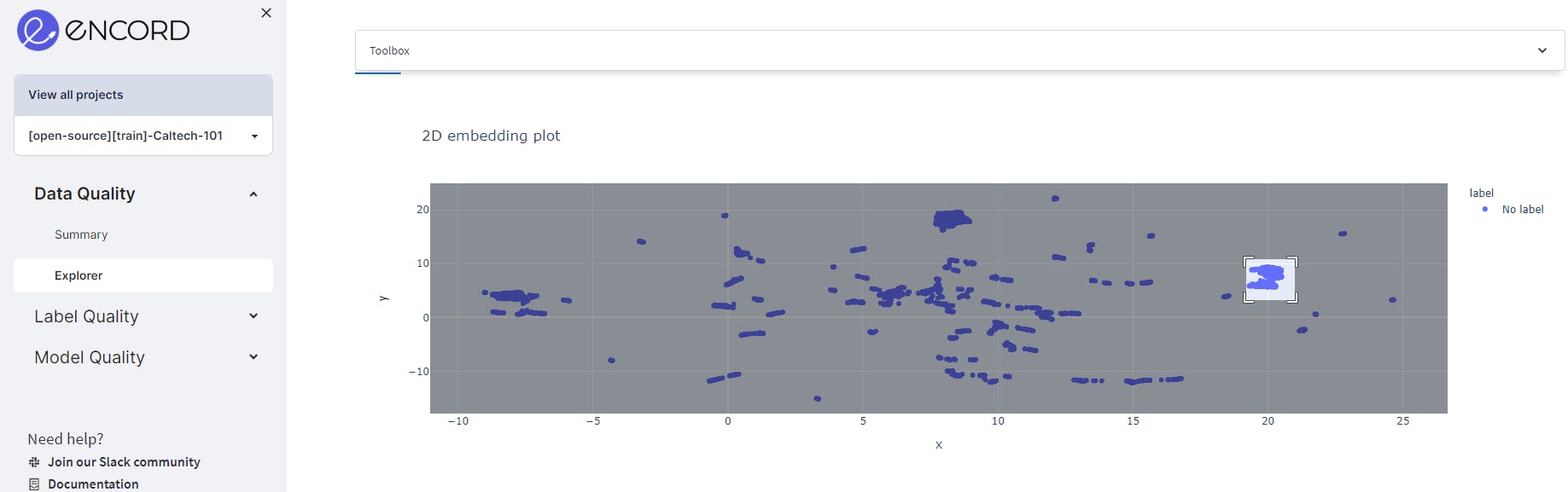
2D embedding plot in Encord Active using the Caltech101 dataset

The use of a 2D embedding plot is to provide an intuitive way of visualizing complex high-dimensional data. It enables the user to observe patterns and relationships that may be difficult to discern in the original high-dimensional space. 

By projecting the data into two dimensions, the user can see clusters of similar data points, outliers, and other patterns that may be useful for data analysis. 

The 2D embedding plot can also be used as a tool for exploratory data analysis, as it allows the user to interactively explore the data and identify interesting subsets of data points. Additionally, the 2D embedding plot can be used as a pre-processing step for machine learning tasks such as classification or clustering, as it can provide a compact representation of the data that can be easily fed into machine learning algorithms.

Area

The area metric is calculated as the product of image width and image height. Here, the plot shows a wide range of image areas, which indicates that the dataset has diverse image sources. It may need pre-processing to normalize or standardize the image values to make them more comparable across different images. 

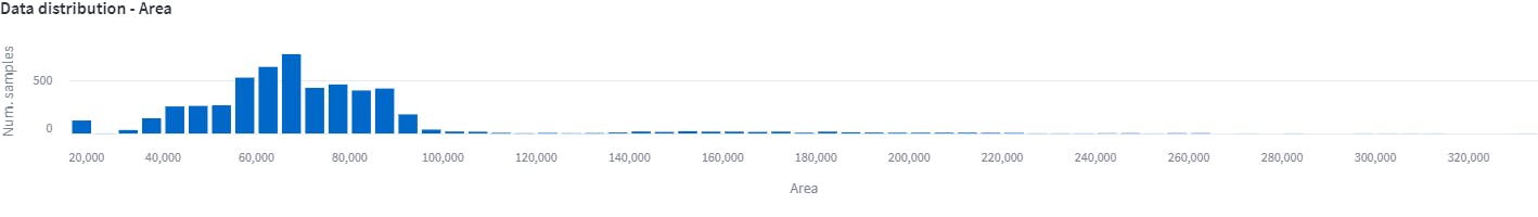
After 100,000 pixels, there are quite a few images.

These images are very large compared to the rest of the dataset. The plot also reveals that after 100,000 pixels, there are few data points. These outliers need to be removed or pre-processed before using them for training.

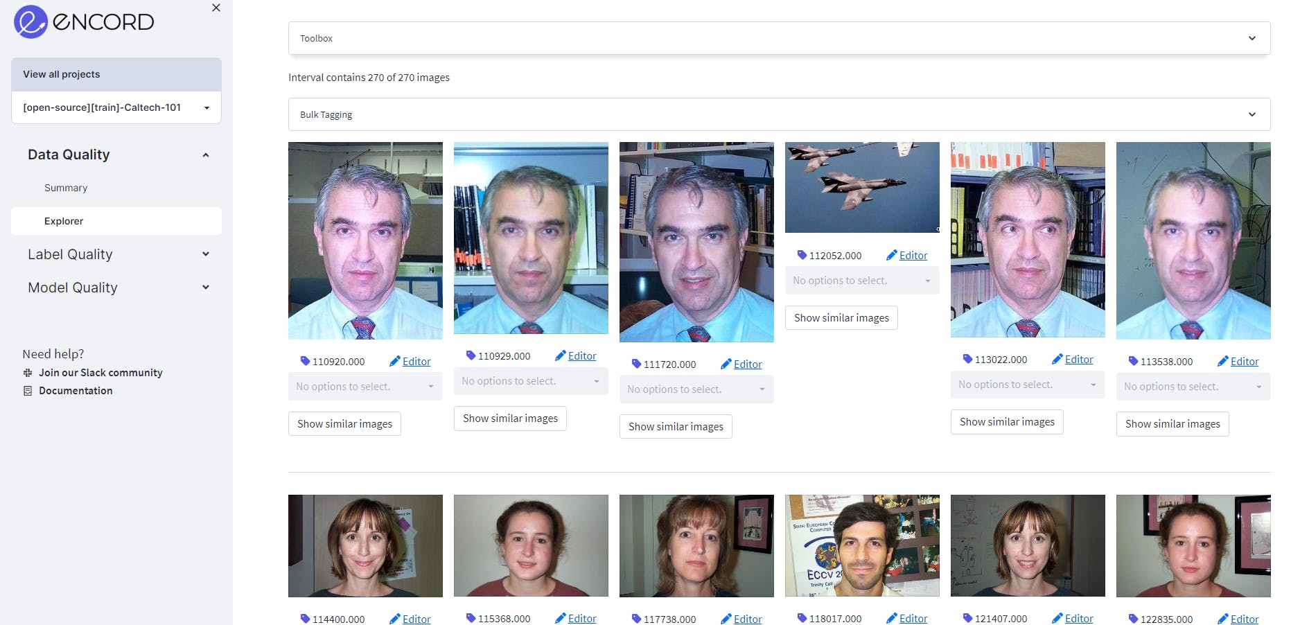
An example of images of people's faces in the dataset, using Encord Active to tag them to assess data quality

Aspect Ratios

Aspect ratio is calculated as the ratio of image width to image height. Here, the data distribution shows that the aspect ratio varies from 0.27 to 3.88. This indicates that the dataset is very diverse. 

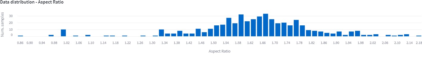
Aspect ratios

The distribution of images with an aspect ratio from 1.34 to 1.98 has the largest density. The rest are the outliers that need to be processed or removed. 

Normalizing the aspect ratios ensures that all images have the same size and shape. This helps in creating a consistent representation of the data which is easier to process and work with. When the aspect ratios are not normalized, the model has to adjust to the varying aspect ratios of the images in the dataset, leading to longer training times. Normalizing the aspect ratios ensures that the model learns from a consistent set of images, leading to faster training times.

Image Singularity

The image singularity metric gives each image a score that shows each image’s uniqueness in the dataset.  A score of zero indicates that the image is a duplicate of another image in the dataset, while a score close to one indicates that the image is more unique, i.e., there are no similar images to that. 

This metric can be useful in identifying duplicate and near-duplicate images in a dataset. Near-duplicate images are images that are not exactly the same but contain the same object which has been shifted/rotated/blurred. Overall, it helps in ensuring that each object is represented from different viewpoints.

Image singularity is important for small datasets like Caltech101 because, in such datasets, each image carries more weight in terms of the information it provides for training the machine learning model so duplicate images may create a bias. When the dataset is small, there are fewer images available for the model to learn from, and it is important to ensure that each image is unique and provides valuable information for the model.

Also, small datasets are more prone to overfitting, which occurs when the model learns to memorize the training data rather than generalize to new data. This can happen if there are too many duplicate or highly similar images in the dataset, as the model may learn to rely on these images rather than learning generalizable features.

By using the image singularity metric to identify and remove duplicate or highly similar images, we can ensure that the small dataset is diverse and representative of the objects or scenes we want the model to recognize. This can help to prevent overfitting and improve the generalizability of the model to new data.

In order to find the exact duplicates, select the image singularity filter and set the score to 0. We observe that the Caltech101 dataset contains 46 exact duplicates. 

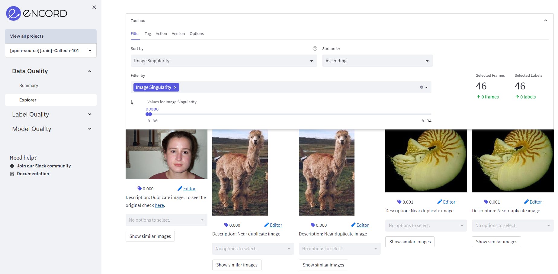
Image singularity metric showing the exact-duplicate images.

Setting the score from 0-0.1, we get the exact duplicates and the near-duplicates. The near-duplicates as also visualized side-by-side so that it is easier to filter them out. Depending on the size of the dataset, it is important to select different thresholds to filter out the near duplicates. For visualization, we have selected a score from 0-0.1 for visualizing near-duplicate images.

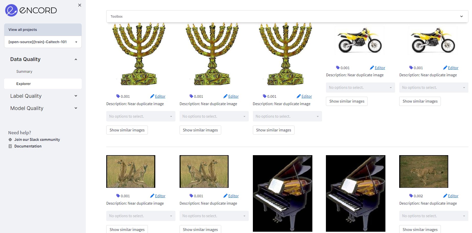
Selecting different thresholds to filter out the near duplicates

The range consists of 3281 images, which accounts for nearly 60% of the training dataset. It's crucial to have these annotations verified by the annotator or machine learning experts to determine whether or not they should be retained in the dataset.

Blur

Blurring an image refers to intentionally or unintentionally reducing the sharpness or clarity of the image, typically by averaging or smoothing nearby pixel values. It is often added for noise reduction or privacy protection.

However, blurred images have negative effects on the performance of object recognition models trained on such images. This is because blur removes or obscures important visual features of objects, making it more difficult for the model to recognize them. 

For example, blurring can remove edges, texture, and other fine-grained details that are important for distinguishing one object from another.

Hence for object recognition models, blur is an important data quality metric. This is because blurring can reduce the image's quality and usefulness for training the model.

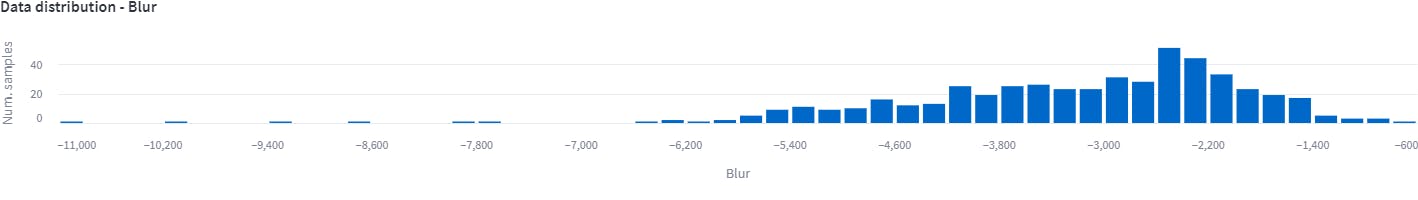
Assessing Blur for data distribution

This data distribution shows blurred images. The blurriness here is computed by applying a Laplacian filter to each image and computing the variance of the output. The distribution above shows that from -1400 to -600 there are few outliers.

By detecting and removing these blurred images from the dataset, we can improve the overall quality of the data used to train the model, which can lead to better model performance and generalization. 

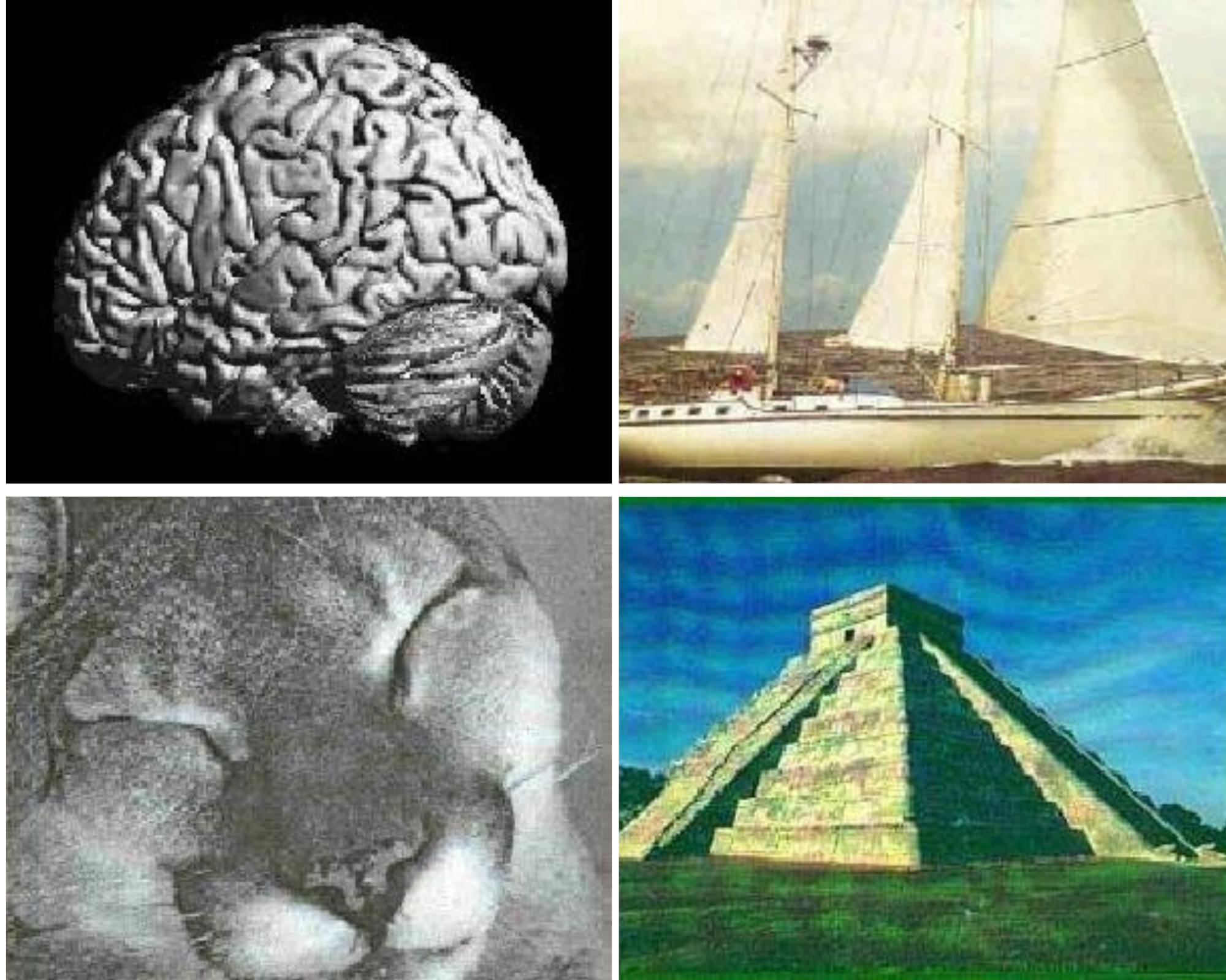
Example of blurred images.

Label Quality of the Caltech 101 Dataset

To assess label quality, we navigate to the Label Quality→Summary tab and check out the overall information about the label quality of the dataset. Information such as object annotations, classification annotations, and the metrics to find the issues in the labels can be found here. 

The summary page of label quality.

The Explorer page has information about the labeled dataset on the metric level. The dataset can be analyzed based on each metric. The metrics which showed as a red flag on the summary page would be a good starting point for the label quality analysis. Navigating to Label Quality→Explorer, gets you to the explorer page. 

Image-level Annotation Quality

The image-level annotation quality metric compares the image classifications against similar objects. This is a ratio where the value 1 shows that the annotation is correct whereas the value between 0-1 indicates a discrepancy in the annotation and the image classification. 

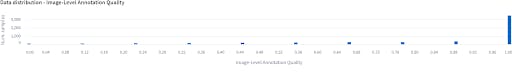
Using the data distribution plot to assess image-level annotation quality

The data distribution plot clearly shows that there are outliers whose image level annotation quality is questionable. 

Setting the filter score between 0-0.01 we get 92 images that have label errors. This is a significant level of label errors. These errors occur due to a variety of reasons such as human error, inconsistencies in labeling criteria, etc. Label errors can affect the quality and accuracy of computer vision models that use the dataset. Incorrect labels can cause the model to learn inaccurate patterns and make inaccurate predictions. With a small dataset like Caltech101, it is important to fix these label errors.

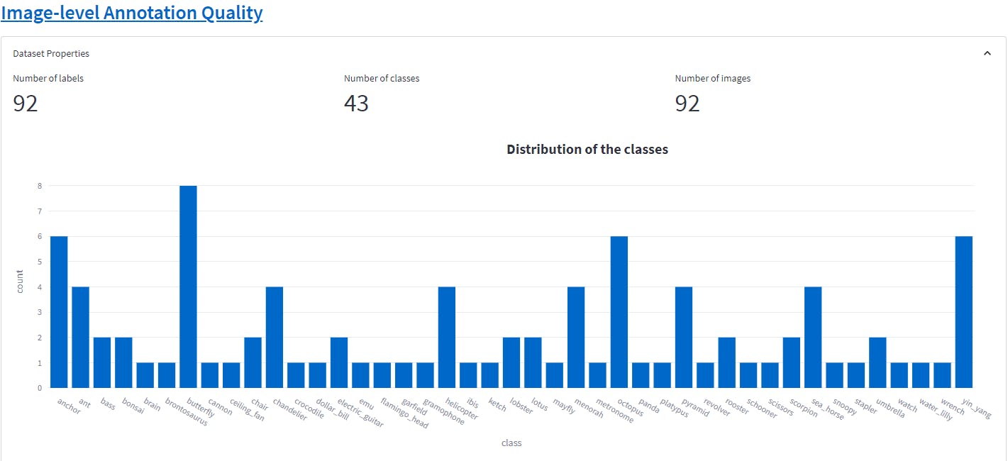
This shows the class-level distribution of the label errors. The class butterfly and yin-gang have the most label errors.

In the above image, we can see how there is a discrepancy between the annotation and what similar objects are tagged in the class butterfly. Having an annotator review these annotations, will improve the label quality of the dataset for building a robust object recognition model.

Object Class Distribution

The distribution of classes plot below so shows that classes like airplanes, faces, watch, and barrels are over-represented in the Caltech101 dataset. The classes below the median are undersampled. Hence, this dataset is imbalanced. Class imbalance can cause problems in any computer vision model because they tend to be biased towards the majority class, resulting in poor performance for the minority class. The model may have high accuracy overall, but it may miss important instances of the minority class, leading to false negatives. 

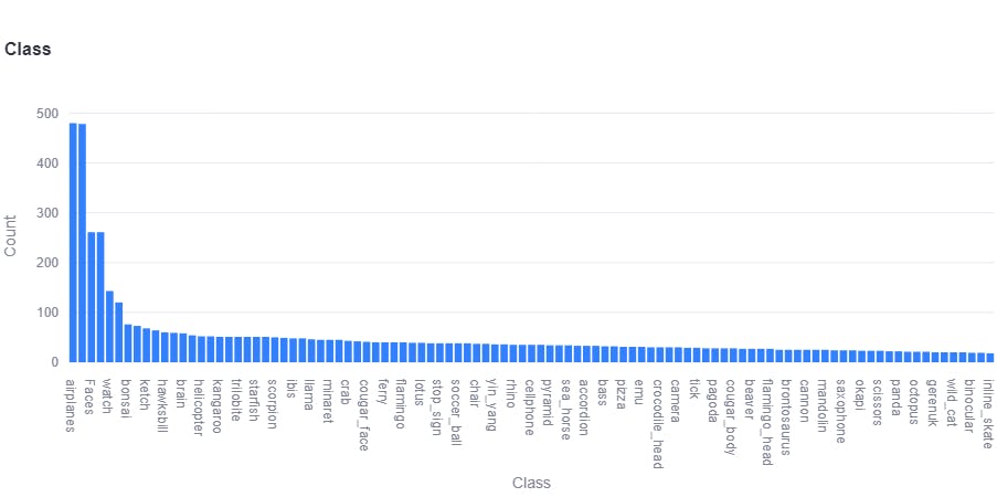
Balancing your computer vision dataset

2D Embeddings

The 2D embedding plot in label quality shows the data points of each image and each color represents the class the object belongs. This helps in finding out the outliers by spotting the unexpected relationships or possible areas of model bias for object labels. 

This plot also shows the separability of the dataset. A separable dataset is useful for object recognition because it allows for the use of simpler and more efficient computer vision models that can achieve high accuracy with relatively few parameters. 

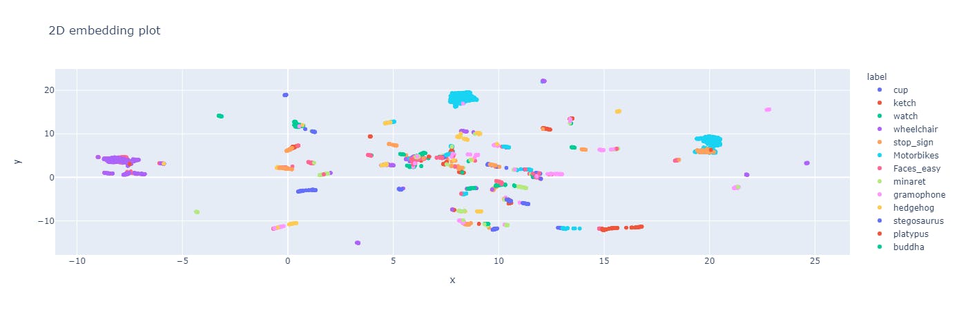
2D embedding plot in label quality

Here, we can see, the different classes of objects are well-defined and can be easily distinguished from each other using a simple decision boundary. Hence, the Caltech 101 dataset is separable.

A separable dataset is a useful starting point for object recognition, as it allows us to quickly develop and evaluate simple machine learning models before exploring more complex models if needed. It also helps us better understand the data and the features that distinguish the different classes of objects, which can be useful for developing more sophisticated models in the future.

Model Quality Analysis

We have trained a benchmark model on the training dataset of Caltech101 and will be evaluating the model's performance on the testing dataset. We need to import the predictions to Encord Active to evaluate the model.

After training the benchmark model, it is natural to be eager to assess its performance. By importing your predictions into Encord Active, the platform will automatically compare your ground truth labels with the predictions and provide you with useful insights about the model’s performance. Some of the information you can obtain includes:

• Class-specific performance results
• Precision-Recall curves for each class, as well as class-specific AP/AR results
• Identification of the 25+ metrics that have the greatest impact on the model’s performance
• Detection of true positive and false positive predictions, as well as false negative ground truth objects

The quality analysis of the model here is done on the test data, which is the 40% of the Caltech101 dataset not used in training. 

Assessing Model Performance Using Caltech 101

The model accuracy comes to 83% on the test dataset. The mean precision comes to 0.75 and the recall of 0.71. This indicates that the object recognition model is performing fairly well, but there is still room for improvement. 

Precision refers to the proportion of true positives out of all the predicted positives, while recall refers to the proportion of true positives out of all the actual positives. A precision of 0.75 means that out of all the objects the model predicted as positive, 75% were actually correct. A recall of 0.71 means that out of all the actual positive objects, the model correctly identified 71% of them.

While an accuracy of 83% may seem good, it’s important to consider the precision and recall values as well. Depending on the context and task requirements, precision and recall may be more important metrics to focus on than overall accuracy.

Assessing Model Performance Using Caltech 101

Performance metrics 

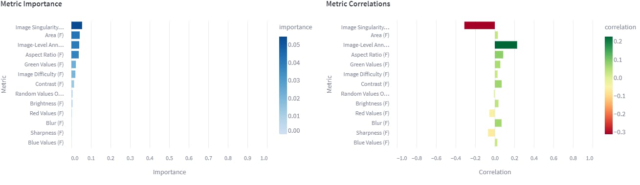
Our initial aim is to examine which quality metrics have an impact on the performance of the model. If a metric holds significant importance, it suggests that any changes in that metric would considerably influence the model’s performance. 

Here we see that image singularity, area, Image-level annotation and aspect ratio are the important metrics.

These metrics affect positively or negatively on the model. For example: 

Image Singularity

Image singularity negatively affects the benchmark model as more images are more unique. Similarly, the model learns object classes with similar images (not exact duplicates). Hence it is harder for the model to learn those patterns.

Area

Image area positively affects the benchmark model. High area values mean that images in the dataset have high resolution. High-resolution images provide more information for the classification model to learn.

On the other hand, if dealing with limited computational resources, these high-resolution images can affect the benchmark model negatively. High-resolution images require large amounts of memory and processing power making them computationally expensive.

Image-level Annotation

This metric is useful to filter out the images which are hard for the model to learn. A low score represents hard images whereas a score close to 1 represents the high-quality annotated images that are easy for the model to learn. The high-quality image-level annotations also have no label errors.

Scale your annotation workflows and power your model performance with data-driven insights

Try Encord today

Precision-Recall

Precision and recall are two common metrics used to evaluate the performance of the computer vision model. Precision measures the proportion of true positives out of all the predicted positives. Recall, on the other hand, measures the proportion of true positives out of all the actual positives. 

Precision and recall are often used together to evaluate the performance of a model. In some cases, a high precision score is more important than recall (e.g., in medical diagnoses where a false positive can be dangerous), while in other cases a high recall score is more important than precision (e.g., in spam detection where missing an important message is worse than having some false positives).

It's worth noting that precision and recall are trade-offs; as one increases, the other may decrease. 

For example, increasing the threshold for positive predictions may increase precision but decrease recall, while decreasing the threshold may increase recall but decrease precision. 

It's important to consider both metrics together and choose a threshold that balances precision and recall based on the specific needs of the problem being solved. We can refer to the average F1 score on the model performance page to consider both metrics. The F1 score is a measure of the model’s precision and recall. The f1 score is computed for each class in the dataset and averaged across all classes. This provides an insight into the performance of the model across all classes.

Scale your annotation workflows and power your model performance with data-driven insights

Try Encord today

The precision-recall plot gives the overview of the precision and recall of all classes of objects in our dataset. We can see some of the classes like “Garfield”, and “binocular”, and others, have huge differences, and hence the threshold need to be balanced for a high-performing model. 

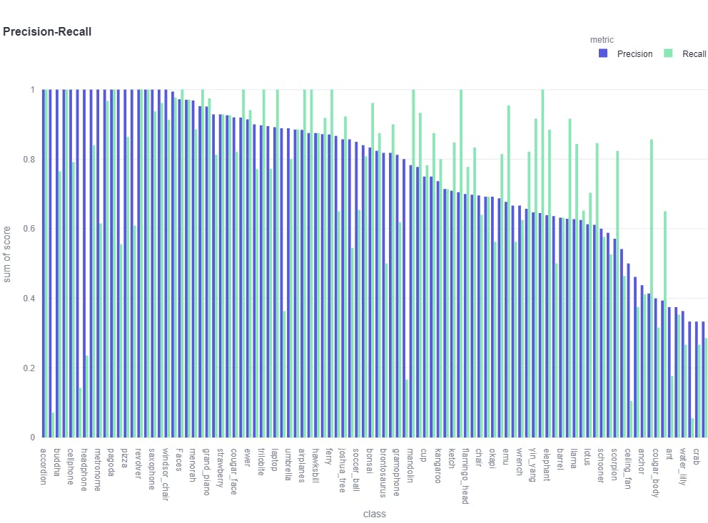
Precision-recall plot

Confusion matrix

A confusion matrix is a table that is often used to evaluate the performance of a machine learning model on a classification task. It summarizes the predicted labels and the actual labels for a set of test data, allowing us to visualize how well the model is performing. 

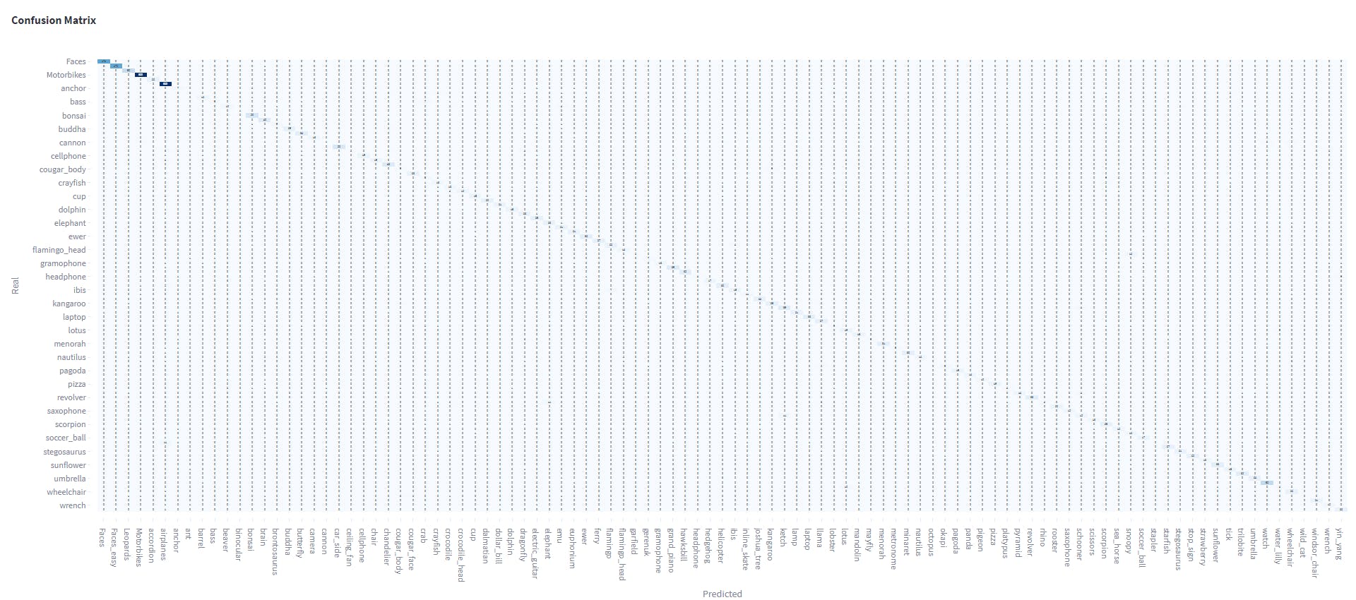
The confusion matrix of the Caltech101 dataset

The confusion matrix of the Caltech101 dataset shows the object classes which are often confused. For example, the image below shows that the class Snoopy and Garfield are often confused with each other.

Object class snoopy is confused with Garfield

Performance By Metric

In the performance by metric tab, as the name suggests we can find the true positive rate of different metrics of the predictions. It indicates the proportion of actual positive cases that are correctly identified as positive by the model. We want the true positive rate to be high in all the important metrics (found in the model performance).

Earlier, we saw that area, image singularity, etc, are some of the important metrics. The plot below shows the predictions' true positive rate with image singularity as a metric.

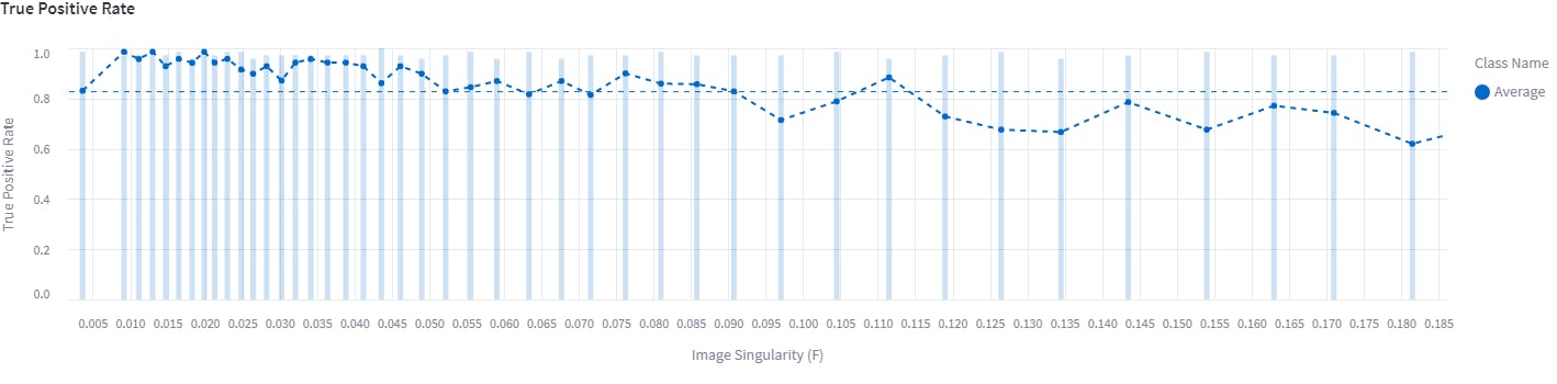
An example of an average true positive rate

The average true positive rate is 0.8 which is a good metric and indicates that the baseline model trained is robust.

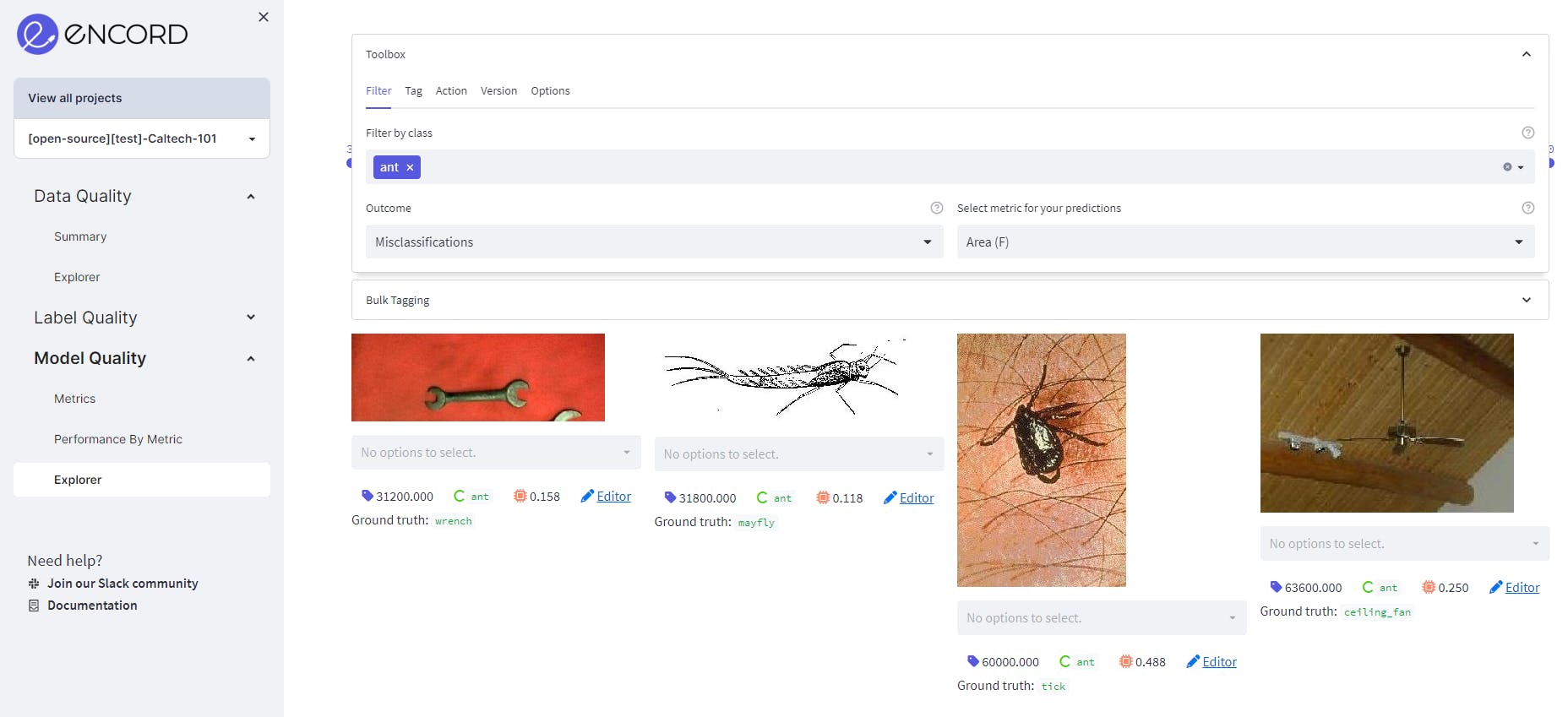
Misclassifications

Going to the Model Quality→Explorer tab, we find the filter to visualize the objects which have been wrongly predicted. 

We can also find out the misclassifications in each class. 

Conclusion

In this blog, we explored the topic of object classification with a focus on the Caltech 101 dataset. We began by discussing the importance of object classification in computer vision and its various applications. We then introduced the Caltech 101 dataset.

We also discussed the importance of data quality in object recognition and evaluated the data quality of the Caltech 101 dataset using the Encord Active tool. We looked at various aspects of data quality, including aspect ratios, image area, blurred images, and image singularity. Furthermore, we evaluated the label quality of the dataset using 2D embedding and image annotation quality.

Next, we trained a benchmark object classification model using the Caltech 101 dataset and analyzed its performance on Encord Active. We also evaluated the quality metrics of the model and identified the misclassified objects in each class. 

Ready to improve the performance and scale your object classification models? 

Sign-up for an Encord Free Trial: The Active Learning Platform for Computer Vision, used by the world’s leading computer vision teams. 

AI-assisted labeling, model training & diagnostics, find & fix dataset errors and biases, all in one collaborative active learning platform, to get to production AI faster. Try Encord for Free Today. 

Want to stay updated?

• Follow us on Twitter and LinkedIn for more content on computer vision, training data, and active learning.
• Join the Slack community to chat and connect.

Further Steps

To further improve the performance of object classification models, there are several possible next steps that can be taken. Firstly, we can explore more sophisticated models that are better suited for the specific characteristics of the Caltech 101 dataset. Additionally, we can try incorporating other datasets or even synthetic data to improve the model's performance.

Another possible direction is to investigate the impact of various hyperparameters, such as learning rate, batch size, and regularization, on the model's performance. We can also experiment with different optimization techniques, such as stochastic gradient descent, Adam, or RMSprop, to see how they affect the model's performance.

Finally, we can explore the use of more advanced evaluation techniques, such as cross-validation or ROC curves, to better understand the model's performance and identify areas for improvement. By pursuing these further steps, we can continue improving the accuracy and robustness of object classification models, which will significantly impact various fields such as medical imaging, autonomous vehicles, and security systems.