Back to Blogs

Contents

What is Time Series Data?
Recurrent Neural Networks (RNNs)
Building and Training the Recurrent Neural Networks (RNNs) Model for Time Series Predictions
Evaluating Model Performance
Limitations of Time Series Predictions with Recurrent Neural Networks (RNNs)
Advanced Techniques and Improvements
Case Study: Applying Recurrent Neural Networks (RNNs) to Real Data
Time Series Predictions with Recurrent Neural Networks (RNNs): Key Takeaways
Time Series Predictions with Recurrent Neural Networks (RNNs): Frequently Asked Questions

Encord Blog

Time Series Predictions with RNNs

August 18, 2023

6 mins

Back to Blogs

Contents

What is Time Series Data?
Recurrent Neural Networks (RNNs)
Building and Training the Recurrent Neural Networks (RNNs) Model for Time Series Predictions
Evaluating Model Performance
Limitations of Time Series Predictions with Recurrent Neural Networks (RNNs)
Advanced Techniques and Improvements
Case Study: Applying Recurrent Neural Networks (RNNs) to Real Data
Time Series Predictions with Recurrent Neural Networks (RNNs): Key Takeaways
Time Series Predictions with Recurrent Neural Networks (RNNs): Frequently Asked Questions

Written by

Nikolaj Buhl

View more posts

Time series prediction, or time series forecasting, is a branch of data analysis and predictive modeling that aims to make predictions about future values based on historical data points in chronological order. In a time series, data is collected and recorded over regular intervals of time (i.e. hourly, daily, monthly, or yearly). Examples of time series data include stock prices, weather measurements, sales figures, website traffic, and more.

Recurrent Neural Networks (RNNs) are deep learning models that can be utilized for time series analysis, with recurrent connections that allow them to retain information from previous time steps. Popular variants include Long Short-Term Memory (LSTM) and Gated Recurrent Unit (GRU), which can learn long-term dependencies.

In this article, you will learn about:

Time Series Data
Recurrent Neural Networks (RNNs)
Building and training the Recurrent Neural Networks (RNN) Model
Evaluating the Model Performance
Limitations of Time Series Predictions with Recurrent Neural Networks (RNNs)
Advanced Techniques for Time Series Predictions
Applying Recurrent Neural Networks (RNNs) on real data (Using Python and Keras)

To learn about activation functions, read: Activation Functions in Neural Networks: With 15 examples.

Build Better Models, Faster with Encord's Leading Annotation Tool

What is Time Series Data?

Time series data is a sequence of observations recorded over time, where each data point is associated with a specific timestamp. This data type is widely used in various fields to analyze trends, make predictions, and understand temporal patterns. Time series data has unique characteristics, such as temporal ordering, autocorrelation (where a data point depends on its previous ones), and seasonality (repeating patterns over fixed intervals).

Recurrent Neural Networks (RNNs) bring a unique edge to time series forecasting, empowering you to capture intricate temporal dependencies. Exploring the realm of Long Short-Term Memory (LSTM) and Gated Recurrent Unit (GRU) models unveils the genuine potential of predictive analytics.

Types of Time Series Patterns

Time series data analysis involves identifying various patterns that provide insights into the underlying dynamics of the data over time. These patterns shed light on the trends, fluctuations, and noise present in the dataset, enabling you to make informed decisions and predictions. Let's explore some of the prominent time series patterns that help us decipher the intricate relationships within the data and leverage them for predictive analytics.

From discerning trends and seasonality to identifying cyclic patterns and understanding the impact of noise, each pattern contributes to our understanding of the data's behavior over time. Additionally, time series regression introduces a predictive dimension, allowing you to forecast numerical values based on historical data and the influence of other variables.

Delving into the below patterns not only offers a world of insights within time-dependent data but also unearths distinct components that shape its narrative:

Trends: Trends represent long-term changes or movements in the data over time. These can be upward (increasing trend) or downward (decreasing trend), indicating the overall direction in which the data is moving.
Seasonality: Seasonality refers to repeating patterns or fluctuations that occur at regular intervals. These patterns might be daily, weekly, monthly, or yearly, depending on the nature of the data.
Cyclic Patterns: Unlike seasonality, cyclic patterns are not fixed to specific intervals and may not repeat at regular frequencies. They represent oscillations that are not tied to a particular season.
Noise: Noise is the random variation present in the data which does not follow any specific pattern. It introduces randomness and uncertainty to the time series.
Regression: Time series regression involves building a predictive model to forecast a continuous numerical value (the dependent variable) based on historical time series data of one or more predictors (independent variables).

Preprocessing Techniques for Time Series Data

Before applying any prediction model, proper preprocessing is essential for time series data. Some common preprocessing techniques include:

Handling Missing Values: Addressing missing values is crucial as gaps in the data can affect the model's performance. You can use techniques like interpolation or forward/backward filling.
Data Normalization: Normalizing the data ensures that all features are on the same scale, preventing any single feature from dominating the model's learning process.
Detrending: Removing the trend component from the data can help in better understanding the underlying patterns and making accurate predictions.
Seasonal Adjustment: For data with seasonality, seasonal adjustment methods like seasonal differencing or seasonal decomposition can be applied.
Smoothing: Smoothing techniques like moving averages can be used to reduce noise and highlight underlying patterns.
Train-test Split: It is crucial to split the data into training and test sets while ensuring that the temporal order is maintained. This allows the model to learn from past input data of the training set and evaluate its performance on unseen future data.

Mastering the train-validation-test split is crucial for robust machine learning models. Learn how to segment datasets effectively, prevent overfitting, and optimize model performance in our comprehensive guide on Training, Validation, and Test Split for Machine Learning Datasets.

With a grasp of the characteristics of time series data and the application of suitable preprocessing methods, you can lay the groundwork for constructing resilient predictive models utilizing Recurrent Neural Networks (RNNs).

Recurrent Neural Networks (RNNs)

A Recurrent Neural Network (RNN) is like a specialized brain for handling sequences, such as sentences or time-based data. Imagine it as a smart cell with its own memory. For example, think about predicting words in a sentence. The RNN not only understands each word but also remembers what came before using its internal memory. This memory helps it capture patterns and relationships in sequences. This makes RNNs great for tasks like predicting future values in time series data, like stock prices or weather conditions, where past information plays a vital role.

Advantages

Recurrent Neural Networks (RNNs) offer several advantages for time series prediction tasks. They can handle sequential data of varying lengths, capturing long-term dependencies and temporal patterns effectively. RNNs accommodate irregularly spaced time intervals and adapt to different forecasting tasks with input and output sequences of varying lengths.

However, RNNs have limitations like the vanishing or exploding gradient problem, which affects their ability to capture long-term dependencies because RNNs may be unrolled very far back in this Memory constraints may also limit their performance with very long sequences. While techniques like LSTMs and GRUs mitigate some issues, other advanced architectures like Transformers might outperform RNNs in certain complex time series scenarios, necessitating careful model selection.

Limitations

The vanishing gradient problem is a challenge that affects the training of deep neural networks, including Recurrent Neural Networks (RNNs). It occurs when gradients, which indicate the direction and magnitude of updates to network weights during training, become very small as they propagate backward through layers. This phenomenon hinders the ability of RNNs to learn long-range dependencies and can lead to slow or ineffective training.

The vanishing gradient problem is particularly problematic in sequences where information needs to be remembered or propagated over a long span of time, affecting the network's ability to capture important patterns. To combat the vanishing gradient problem that hampers effective training in neural networks, several strategies have emerged. Techniques like proper weight initialization, batch normalization, gradient clipping, skip connections, and learning rate scheduling play pivotal roles in stabilizing gradient flow and preventing their untimely demise.

Amid this spectrum of approaches, two standout solutions take center stage: LSTM (Long Short-Term Memory) and GRU (Gated Recurrent Unit).

Long Short-Term Memory (LSTM) and Gated Recurrent Unit (GRU)

Traditional RNNs struggle with the vanishing gradient problem, which makes it difficult for the network to identify long-term dependencies in sequential data. However, this challenge is elegantly addressed by LSTM, as it incorporates specialized memory cells and gating mechanisms that preserve and control the flow of gradients over extended sequences. This enables the network to capture long-term dependencies more effectively and significantly enhances its ability to learn from sequential data. LSTM has three gates (input, forget, and output) and excels at capturing long-term dependencies.

Gated Recurrent Unit (GRU), a simplified version of LSTM with two gates (reset and update), maintains efficiency and performance similar to LSTM, making it widely used in time series tasks.

In 1997, Sepp Hochreiter and Jürgen Schmidhuber published a seminal paper titled "Long Short-Term Memory" that introduced the LSTM network. Both the scientists are pioneers in the field of Artificial Intelligence and Machine Learning.

Building and Training the Recurrent Neural Networks (RNNs) Model for Time Series Predictions

Building and training an effective RNN model for time series predictions requires an approach that balances model architecture and training techniques. This section explores all the essential steps for building and training an RNN model. The process includes data preparation, defining the model architecture, building the model, fine-tuning hyperparameters, and then evaluating the model’s performance.

Data Preparation

Data preparation is crucial for accurate time series predictions with RNNs. Handling missing values and outliers, scaling data, and creating appropriate input-output pairs are essential. Seasonality and trend removal help uncover patterns, while selecting the right sequence length balances short- and long-term dependencies.

Feature engineering, like lag features, improves model performance. Proper data preprocessing ensures RNNs learn meaningful patterns and make accurate forecasts on unseen data.

Building the RNN Model

Building the RNN model includes a series of pivotal steps that collectively contribute to the model’s performance and accuracy.

Designing the RNN Architecture: Constructing the RNN architecture involves deciding the layers and the neurons in the network. A typical structure for time series prediction comprises an input layer, one or more hidden layers with LSTM or GRU cells and an output layer.
Selecting the optimal number of layers and neurons: This is a critical step in building the RNN model. Too few layers or neurons may lead to underfitting, while too many can lead to overfitting. It's essential to strike a balance between model complexity and generalization. You can use techniques like cross-validation and grid search to find the optimal hyperparameters.
Hyperparameter tuning and optimization techniques: Hyperparameter tuning involves finding the best set of hyperparameters for the RNN model. Hyperparameters include learning rate, batch size, number of epochs, and regularization strength. You can employ grid or randomized search to explore different combinations of hyperparameters and identify the configuration that yields the best performance.

Hyperparameter Tuning

Training the Recurrent Neural Networks (RNNs) Model

Training an RNN involves presenting sequential data with learning algorithms to the model and updating its parameters iteratively to minimize the prediction error.

By feeding historical sequences into the RNN, it learns to capture patterns and dependencies in the data. The process usually involves forward propagation to compute predictions and backward propagation to update the model's weights using optimization algorithms like Stochastic Gradient Descent (SGD) or Adam.

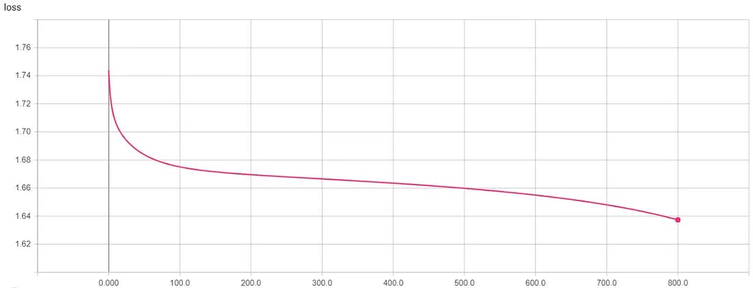
Time series predictions with recurrent neural networks (RNN) - SGD

Stochastic Gradient Descent, Learning Rate = 0.01

Backpropagation through time (BPTT) is a variant of the standard backpropagation algorithm used in RNNs.

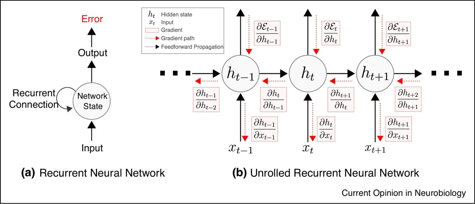
Time series predictions with recurrent neural networks - bptt

Backpropagation through time (BPTT)

Overfitting is a common issue in deep learning models, including RNNs. You can employ regularization techniques like L1 and L2 regularization, dropout, and early stopping to prevent overfitting and improve the model's generalization performance.

Evaluating Model Performance

To assess the performance of the trained RNN model, you can use evaluation metrics such as Mean Absolute Error (MAE), Root Mean Squared Error (RMSE), and Mean Absolute Percentage Error (MAPE). These metrics quantify the accuracy of the predictions compared to the actual values and provide valuable insights into the model's effectiveness.

Visualizing the model's predictions against the actual time series data can help you understand its strengths and weaknesses. Plotting the predicted values alongside the true values provides an intuitive way to identify patterns, trends, and discrepancies. Interpreting the results involves analyzing the evaluation metrics, visualizations, and any patterns or trends observed.

Based on the analysis, you can identify potential improvements to the model. These may include further tuning hyperparameters, adjusting the architecture, or exploring different preprocessing techniques. By carefully building, training, and evaluating the RNN model, you can develop a powerful tool for time series prediction that can capture temporal dependencies and make accurate forecasts.

Limitations of Time Series Predictions with Recurrent Neural Networks (RNNs)

While Recurrent Neural Networks (RNNs) offer powerful tools for time series predictions, they have certain limitations. Understanding these limitations is crucial for developing accurate and reliable predictive models. RNNs may struggle with capturing long-term dependencies, leading to potential prediction inaccuracies.

Additionally, training deep RNNs can be computationally intensive, posing challenges for real-time applications. Addressing these limitations through advanced architectures and techniques is essential to harnessing the full potential of RNNs in time series forecasting.

Non-Stationary Time Series Data

Non-stationary time series data exhibits changing statistical properties such as varying mean or variance, over time. Dealing with non-stationarity is crucial, as traditional models assume stationarity.

Techniques like differencing, detrending, or seasonal decomposition can help transform the data into a stationary form. Additionally, advanced methods like Seasonal Autoregressive Integrated Moving Average (SARIMA) or Prophet can be used to model and forecast non-stationary time series.

Data with Irregular Frequencies and Missing Timestamps

Real-world time series data can have irregular frequencies and missing timestamps, disrupting the model's ability to learn patterns. You can apply resampling techniques (e.g., interpolation, aggregation) to convert data to a regular frequency. For missing timestamps, apply imputation techniques like forward and backward filling or more advanced methods like time series imputation models.

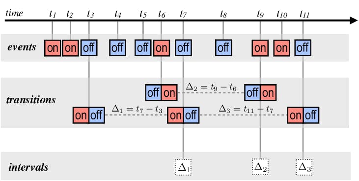
Time series predictions with recurrent neural networks (RNNs) - time series data

Time series data: a single pixel produces an irregular series of raw events

Concept Drift and Model Adaptation

In dynamic environments, time series data might undergo concept drift, where the underlying patterns and relationships change over time. To address this, the model needs to adapt continuously. Use techniques like online learning and concept drift detection algorithms to monitor data distribution changes and trigger model updates when necessary.

Advanced Techniques and Improvements

As time series data becomes more complex and diverse, advanced techniques are essential to enhance the capabilities of Recurrent Neural Networks (RNNs). Multi-variate time series data featuring multiple interconnected variables can be effectively handled by extending RNNs to accommodate multiple input features and output predictions. Incorporating attention mechanisms refines RNN predictions by prioritizing relevant time steps or features, especially in longer sequences.

Also, combining RNNs with other models like CNN-RNN, Transformer-RNN, or ANN-RNN makes hybrid architectures that can handle both spatial and sequential patterns. This improves the accuracy of predictions in many different domains. These sophisticated techniques empower RNNs to tackle intricate challenges and deliver comprehensive insights.

Multi-Variate Time Series Data in Recurrent Neural Networks (RNNs)

In many real-world scenarios, time series data may involve multiple related variables. You can extend RNNs to handle multi-variate time series by incorporating multiple input features and predicting multiple output variables. This allows the model to leverage additional information to make more accurate predictions and better capture complex relationships among different variables.

Time series predictions with recurrent neural networks - Multivariate time series

Multivariate Time Series

Attention Mechanisms for More Accurate Predictions

Attention mechanisms enhance RNNs by focusing on relevant time steps or features during predictions. They improve accuracy and interpretability, especially in long sequences. Combining RNNs with other models, like the convolutional neural network model CNN-RNN or Transformer-RNN, Artificial Neural Networks ANN-RNN, may further boost performance for time series tasks.

ANNs consist of interconnected artificial neurons, nodes or units, organized into layers. Hybrid models effectively handle spatial and sequential patterns, leading to better domain predictions and insights. Advanced techniques like Seq-2-Seq, bidirectional, transformers etc. make RNNs more adaptable, addressing real-world challenges and yielding comprehensive results.

Case Study: Applying Recurrent Neural Networks (RNNs) to Real Data

This case study uses Recurrent Neural Networks (RNNs) to predict electricity consumption based on historical data. The "Electricity Consumption'' dataset contains hourly electricity consumption data over a period of time. The aim is to build an RNN model to forecast future electricity consumption, leveraging past consumption patterns.

Python Code (using Pytorch):

import numpy as np
import pandas as pd
import matplotlib.pyplot as plt
from sklearn.preprocessing import MinMaxScaler
import torch
import torch.nn as nn
from torch.utils.data import DataLoader, Dataset
from sklearn.metrics import mean_absolute_error, mean_absolute_percentage_error, mean_squared_error

# Sample data for Electricity Consumption 
data = {
    'timestamp': pd.date_range(start='2023-01-01', periods=100, freq='H'),
    'consumption': np.random.randint(100, 1000, 100)
}
df = pd.DataFrame(data)
df.set_index('timestamp', inplace=True)

# Preprocessing
scaler = MinMaxScaler()
df_scaled = scaler.fit_transform(df)

# Create sequences and labels for training
seq_length = 24
X, y = [], []
for i in range(len(df_scaled) - seq_length):
    X.append(df_scaled[i:i + seq_length])
    y.append(df_scaled[i + seq_length])


X, y = np.array(X), np.array(y)

# Split the data into training and test sets
train_size = int(0.8 * len(X))
X_train, X_test = X[:train_size], X[train_size:]
y_train, y_test = y[:train_size], y[train_size:]

# Create a custom dataset class for PyTorch DataLoader
class TimeSeriesDataset(Dataset):
    def __init__(self, X, y):
        self.X = torch.tensor(X, dtype=torch.float32)
        self.y = torch.tensor(y, dtype=torch.float32)

    def __len__(self):
        return len(self.X)

    def __getitem__(self, index):
        return self.X[index], self.y[index]

# Define the RNN model
class RNNModel(nn.Module):
    def __init__(self, input_size, hidden_size, output_size):
        super(RNNModel, self).__init__()
        self.rnn = nn.LSTM(input_size, hidden_size, batch_first=True)
        self.fc = nn.Linear(hidden_size, output_size)

    def forward(self, x):
        out, _ = self.rnn(x)
        out = self.fc(out[:, -1, :])
        return out

# Hyperparameters
input_size = X_train.shape[2]
hidden_size = 128
output_size = 1
learning_rate = 0.001
num_epochs = 50
batch_size = 64

# Create data loaders
train_dataset = TimeSeriesDataset(X_train, y_train)
train_loader = DataLoader(train_dataset, batch_size=batch_size, shuffle=True)

# Initialize the model, loss function, and optimizer
model = RNNModel(input_size, hidden_size, output_size)
criterion = nn.MSELoss()
optimizer = torch.optim.Adam(model.parameters(), lr=learning_rate)

# Training the model
for epoch in range(num_epochs):
    for inputs, targets in train_loader:
        outputs = model(inputs)
        loss = criterion(outputs, targets)
        optimizer.zero_grad()
        loss.backward()
        optimizer.step()

  if (epoch + 1) % 10 == 0:
        print(f'Epoch [{epoch+1}/{num_epochs}], Loss: {loss.item():.4f}')

# Evaluation on the test set
model.eval()
with torch.no_grad():
    X_test_tensor = torch.tensor(X_test, dtype=torch.float32)
    y_pred = model(X_test_tensor).numpy()
    y_pred = scaler.inverse_transform(y_pred)
    y_test = scaler.inverse_transform(y_test)

# Calculate RMSE
mse = mean_squared_error(y_test, y_pred)
rmse = np.sqrt(mse)
print(f"Root Mean Squared Error (RMSE): {rmse}")
mae = mean_absolute_error(y_test, y_pred)
print(f"Mean Absolute Error (MAE): {mae:.2f}")
mape = mean_absolute_percentage_error(y_test, y_pred) * 100
print(f"Mean Absolute Percentage Error (MAPE): {mape:.2f}%")


# Visualize predictions against actual data
plt.figure(figsize=(10, 6))
plt.plot(df.index[train_size+seq_length:], y_test, label='Actual')
plt.plot(df.index[train_size+seq_length:], y_pred, label='Predicted')
plt.xlabel('Timestamp')
plt.ylabel('Electricity Consumption')
plt.title('Electricity Consumption Prediction using RNN (PyTorch)')
plt.legend()
plt.show()

Time Series with Recurrent Neural Networks RNN - Github

The provided code demonstrates the implementation of a Recurrent Neural Network (RNN) using PyTorch for electricity consumption prediction. The model is trained and evaluated on a sample dataset. The training process includes 50 epochs, and the loss decreases over iterations, indicating the learning process.

The analysis reveals significant gaps between predicted and actual electricity consumption values, as indicated by the relatively high Root Mean Squared Error (RMSE), Mean Absolute Error (MAE), and Mean Absolute Percentage Error (MAPE). These metrics collectively suggest that the current model's predictive accuracy requires improvement. The deviations underscore that the model falls short in capturing the true consumption patterns accurately.

In the context of the case study, where the goal is to predict electricity consumption using Recurrent Neural Networks (RNNs), these results highlight the need for further fine-tuning.

Despite leveraging historical consumption data and the power of RNNs, the model's performance indicates a discrepancy between predicted and actual values. The implication is that additional adjustments to the model architecture, hyperparameters, or preprocessing of the dataset are crucial. Enhancing these aspects could yield more reliable predictions, ultimately leading to a more effective tool for forecasting future electricity consumption patterns.

"RNNs have revolutionized time series analysis, enabling us to predict future values with remarkable accuracy. Through the lens of LSTM and GRU, you can decipher hidden patterns within temporal data, paving the way for transformative insights in diverse industries." - Dr. John Smith

Time Series Predictions with Recurrent Neural Networks (RNNs): Key Takeaways

Time series data possesses unique characteristics, necessitating specialized techniques for analysis and forecasting.
Recurrent Neural Networks (RNNs) excel in handling sequences, capturing dependencies, and adapting to diverse tasks.
Proper data preparation, model building, and hyperparameter tuning are crucial for successful RNN implementation.
Evaluation metrics and visualization aid in assessing model performance and guiding improvements.
Addressing real-world challenges requires advanced techniques like attention mechanisms and hybrid models.

Time Series Predictions with Recurrent Neural Networks (RNNs): Frequently Asked Questions

What is time series data?

Time series data is a sequence of observations recorded over time, often used in fields like finance and weather forecasting. Its uniqueness lies in temporal ordering, autocorrelation, seasonality, cyclic patterns, and noise, which necessitate specialized techniques for analysis and prediction.

What are recurrent neural networks (RNNs) and their advantages?

RNNs are specialized neural networks designed for sequential data analysis. They excel in handling varying sequence lengths, capturing long-term dependencies, and adapting to irregular time intervals. RNNs are proficient in tasks requiring an understanding of temporal relationships.

How do LSTM and GRU models address challenges like the vanishing gradient problem?

Long Short-Term Memory (LSTM) and Gated Recurrent Unit (GRU) models are RNN variations that mitigate the vanishing gradient problem. They incorporate gating mechanisms that allow them to retain information from previous time steps, enabling the learning of long-term dependencies.

What challenges do recurrent neural networks (RNNs) face, and how can they be overcome?

While RNNs offer powerful capabilities, they also have limitations, including computational demands and potential struggles with very long sequences. Addressing these challenges requires meticulous hyperparameter tuning, careful data preparation, and techniques like regularization.

How can recurrent neural networks (RNNs) be applied to real-world time series data?

Applying RNNs to real-world time series data involves a comprehensive process. It begins with proper data preprocessing, designing the RNN architecture, tuning hyperparameters, and training the model. Evaluation metrics and visualization are used to assess performance and guide improvements, addressing challenges like non-stationarity, missing timestamps, and more.

Scale your annotation workflows and power your model performance with data-driven insights

Build better ML models with Encord

Get started today

Written by

Nikolaj Buhl

View more posts

Frequently asked questions

Time series data is a sequence of observations recorded over time, often used in fields like finance and weather forecasting. Its uniqueness lies in temporal ordering, autocorrelation, seasonality, cyclic patterns, and noise, which necessitate specialized techniques for analysis and prediction.
Applying RNNs to real-world time series data involves a comprehensive process. It begins with proper data preprocessing, designing the RNN architecture, tuning hyperparameters, and training the model. Evaluation metrics and visualization are used to assess performance and guide improvements, addressing challenges like non-stationarity, missing timestamps, and more.
While RNNs offer powerful capabilities, they also have limitations, including computational demands and potential struggles with very long sequences. Addressing these challenges requires meticulous hyperparameter tuning, careful data preparation, and techniques like regularization.
Long Short-Term Memory (LSTM) and Gated Recurrent Unit (GRU) models are RNN variations that mitigate the vanishing gradient problem. They incorporate gating mechanisms that allow them to retain information from previous time steps, enabling the learning of long-term dependencies.
RNNs are specialized neural networks designed for sequential data analysis. They excel in handling varying sequence lengths, capturing long-term dependencies, and adapting to irregular time intervals. RNNs are proficient in tasks requiring an understanding of temporal relationships.

Previous blog

9 Best Image Annotation Tools for Computer Vision of 2023 Compared [Updated]

Next blog

Dual-Stream Diffusion Net for Text-to-Video Generation

May 11 2023

5 M

machine learning

machine learning

Guide to Image Segmentation in Computer Vision: Best Practices

Image segmentation is a crucial task in computer vision, where the goal is to divide an image into different meaningful and distinguishable regions or objects. It is a fundamental task in various applications such as object recognition, tracking, and detection, medical imaging, and robotics. Many techniques are available for image segmentation, ranging from traditional methods to deep learning-based approaches. With the advent of deep learning, the accuracy and efficiency of image segmentation have improved significantly. In this guide, we will discuss the basics of image segmentation, including different types of segmentation, applications, and various techniques used for image segmentation, including traditional, deep learning, and foundation model techniques. We will also cover evaluation metrics and datasets for evaluating image segmentation algorithms and future directions in image segmentation. By the end of this guide, you will have a better understanding of image segmentation, its applications, and the various techniques used for segmenting images. This guide is for you if you are a data scientist, machine learning engineer or your team is considering using image segmentation as part of an artificial intelligence computer vision project. What is Image Segmentation? Image segmentation is the process of dividing an image into multiple meaningful and homogeneous regions or objects based on their inherent characteristics, such as color, texture, shape, or brightness. Image segmentation aims to simplify and/or change the representation of an image into something more meaningful and easier to analyze. Here, each pixel is labeled. All the pixels belonging to the same category have a common label assigned to them. The task of segmentation can further be done in two ways: Similarity: As the name suggests, the segments are formed by detecting similarity between image pixels. It is often done by thresholding (see below for more on thresholding). Machine learning algorithms (such as clustering) are based on this type of approach for image segmentation. Discontinuity: Here, the segments are formed based on the change of pixel intensity values within the image. This strategy is used by line, point, and edge detection techniques to obtain intermediate segmentation results that may be processed to obtain the final segmented image. Types of Segmentation Image segmentation modes are divided into three categories based on the amount and type of information that should be extracted from the image: Instance, semantic, and panoptic. Let’s look at these various modes of image segmentation methods. Also, to understand the three modes of image segmentation, it would be more convenient to know more about objects and backgrounds. Objects are the identifiable entities in an image that can be distinguished from each other by assigning unique IDs, while the background refers to parts of the image that cannot be counted, such as the sky, water bodies, and other similar elements. By distinguishing between objects and backgrounds, it becomes easier to understand the different modes of image segmentation and their respective applications. Instance Segmentation Instance segmentation is a type of image segmentation that involves detecting and segmenting each object in an image. It is similar to object detection but with the added task of segmenting the object’s boundaries. The algorithm has no idea of the class of the region, but it separates overlapping objects. Instance segmentation is useful in applications where individual objects need to be identified and tracked. Instance segmentation Semantic Segmentation Semantic segmentation is a type of image segmentation that involves labeling each pixel in an image with a corresponding class label with no other information or context taken into consideration. The goal is to assign a label to every pixel in the image, which provides a dense labeling of the image. The algorithm takes an image as input and generates a segmentation map where the pixel value (0,1,...255) of the image is transformed into class labels (0,1,...n). It is useful in applications where identifying the different classes of objects on the road is important. Semantic segmentation - the human and the dog are classified together as mammals and separated from the rest of the background. Panoptic Segmentation Panoptic segmentation is a combination of semantic and instance segmentation. It involves labeling each pixel with a class label and identifying each object instance in the image. This mode of image segmentation provides the maximum amount of high-quality granular information from machine learning algorithms. It is useful in applications where the computer vision model needs to detect and interact with different objects in its environment, like an autonomous robot. Panoptic segmentation Each type of segmentation has its unique characteristics and is useful in different applications. In the following section, let’s discuss the various applications of image segmentation. Image Segmentation Techniques Traditional Techniques Traditional image segmentation techniques have been used for decades in computer vision to extract meaningful information from images. These techniques are based on mathematical models and algorithms that identify regions of an image with common characteristics, such as color, texture, or brightness. Traditional image segmentation techniques are usually computationally efficient and relatively simple to implement. They are often used for applications that require fast and accurate segmentation of images, such as object detection, tracking, and recognition. In this section, we will explore some of the most common techniques. Thresholding Thresholding Thresholding is one of the simplest image segmentation methods. Here, the pixels are divided into classes based on their histogram intensity which is relative to a fixed value or threshold. This method is suitable for segmenting objects where the difference in pixel values between the two target classes is significant. In low-noise images, the threshold value can be kept constant, but with images with noise, dynamic thresholding performs better. In thresholding-based segmentation, the greyscale image is divided into two segments based on their relationship to the threshold value, producing binary images. Algorithms like contour detection and identification work on these binarized images. The two commonly used thresholding methods are: Global thresholding is a technique used in image segmentation to divide images into foreground and background regions based on pixel intensity values. A threshold value is chosen to separate the two regions, and pixels with intensity values above the threshold are assigned to the foreground region and those below the threshold to the background region. This method is simple and efficient but may not work well for images with varying illumination or contrast. In those cases, adaptive thresholding techniques may be more appropriate. Adaptive thresholding is a technique used in image segmentation to divide an image into foreground and background regions by adjusting the threshold value locally based on the image characteristics. The method involves selecting a threshold value for each smaller region or block, based on the statistics of the pixel values within that block. Adaptive thresholding is useful for images with non-uniform illumination or varying contrast and is commonly used in document scanning, image binarization, and image segmentation. The choice of adaptive thresholding technique depends on the specific application requirements and image characteristics. Image showing different thresholding techniques. Source: Author Region-based Segmentation Region-based segmentation is a technique used in image processing to divide an image into regions based on similarity criteria, such as color, texture, or intensity. The method involves grouping pixels into regions or clusters based on their similarity and then merging or splitting regions until the desired level of segmentation is achieved. The two commonly used region-based segmentation techniques are: Split and merge segmentation is a region-based segmentation technique that recursively divides an image into smaller regions until a stopping criterion is met and then merges similar regions to form larger regions. The method involves splitting the image into smaller blocks or regions and then merging adjacent regions that meet certain similarity criteria, such as similar color or texture. Split and merge segmentation is a simple and efficient technique for segmenting images, but it may not work well for complex images with overlapping or irregular regions. Graph-based segmentation is a technique used in image processing to divide an image into regions based on the edges or boundaries between regions. The method involves representing the image as a graph, where the nodes represent pixels, and the edges represent the similarity between pixels. The graph is then partitioned into regions by minimizing a cost function, such as the normalized cut or minimum spanning tree. Example of graph-based image segmentation. Source Edge-based Segmentation Edge-based segmentation is a technique used in image processing to identify and separate the edges of an image from the background. The method involves detecting the abrupt changes in intensity or color values of the pixels in the image and using them to mark the boundaries of the objects. The two most common edge-based segmentation techniques are: Canny edge detection is a popular method for edge detection that uses a multi-stage algorithm to detect edges in an image. The method involves smoothing the image using a Gaussian filter, computing the gradient magnitude and direction of the image, applying non-maximum suppression to thin the edges, and using hysteresis thresholding to remove weak edges. Example of canny edge detection Sobel edge detection is a method for edge detection that uses a gradient-based approach to detect edges in an image. The method involves computing the gradient magnitude and direction of the image using a Sobel operator, which is a convolution kernel that extracts horizontal and vertical edge information separately. Example of Sobel edge detection. Laplacian of Gaussian (LoG) edge detection is a method for edge detection that combines Gaussian smoothing with the Laplacian operator. The method involves applying a Gaussian filter to the image to remove noise and then applying the Laplacian operator to highlight the edges. LoG edge detection is a robust and accurate method for edge detection, but it is computationally expensive and may not work well for images with complex edges. Example of Laplacian of Gaussian edge detection. Clustering Clustering is one of the most popular techniques used for image segmentation, as it can group pixels with similar characteristics into clusters or segments. The main idea behind clustering-based segmentation is to group pixels into clusters based on their similarity, where each cluster represents a segment. This can be achieved using various clustering algorithms, such as K means clustering, mean shift clustering, hierarchical clustering, and fuzzy clustering. K-means clustering is a widely used clustering algorithm for image segmentation. In this approach, the pixels in an image are treated as data points, and the algorithm partitions these data points into K clusters based on their similarity. The similarity is measured using a distance metric, such as Euclidean distance or Mahalanobis distance. The algorithm starts by randomly selecting K initial centroids, and then iteratively assigns each pixel to the nearest centroid and updates the centroids based on the mean of the assigned pixels. This process continues until the centroids converge to a stable value. ‍ Showing the result of segmenting the image at k=2,4,10. Source Mean shift clustering is another popular clustering algorithm used for image segmentation. In this approach, each pixel is represented as a point in a high-dimensional space, and the algorithm shifts each point toward the direction of the local density maximum. This process is repeated until convergence, where each pixel is assigned to a cluster based on the nearest local density maximum. Source ‍Though these techniques are simple, they are fast and memory efficient. But these techniques are more suitable for simpler segmentation tasks as well. They often require tuning to customize the algorithm as per the use case and also provide limited accuracy on complex scenes. Deep Learning Techniques Neural networks also provide solutions for image segmentation by training neural networks to identify which features are important in an image, rather than relying on customized functions like in traditional algorithms. Neural nets that perform the task of segmentation typically use an encoder-decoder structure. The encoder extracts features of an image through narrower and deeper filters. If the encoder is pre-trained on a task like an image or face recognition, it then uses that knowledge to extract features for segmentation (transfer learning). The decoder then over a series of layers inflates the encoder’s output into a segmentation mask resembling the pixel resolution of the input image. The basic architecture of the neural network model for image segmentation. Source ‍ Many deep learning models are quite adept at performing the task of segmentation reliably. Let’s have a look at a few of them: U-Net U-Net is a modified, fully convolutional neural network. It was primarily proposed for medical purposes, i.e., to detect tumors in the lungs and brain. It has the same encoder and decoder. The encoder is used to extract features using a shortcut connection, unlike in fully convolutional networks, which extract features by upsampling. The shortcut connection in the U-Net is designed to tackle the problem of information loss. In the U-Net architecture, the encoders and decoders are designed in such a manner that the network captures finer information and retains more information by concatenating high-level features with low-level ones. This allows the network to yield more accurate results. U-Net Architecture. Source‍ SegNet SegNet is also a deep fully convolutional network that is designed especially for semantic pixel-wise segmentation. Like U-Net, SegNet’s architecture also consists of encoder and decoder blocks. The SegNet differs from other neural networks in the way it uses its decoder for upsampling the features. The decoder network uses the pooling indices computed in the max-pooling layer which in turn makes the encoder perform non-linear upsampling. This eliminates the need for learning to upsample. SegNet is primarily designed for scene-understanding applications. SegNet Architecture. Source DeepLab DeepLab is primarily a convolutional neural network (CNN) architecture. Unlike the other two networks, it uses features from every convolutional block and then concatenates them to their deconvolutional block. The neural network uses the features from the last convolutional block and upsamples it like the fully convolutional network (FCN). It uses the atrous convolution or dilated convolution method for upsampling. The advantage of atrous convolution is that the computation cost is reduced while capturing more information. The encoder-Decoder architecture of DeepLab v3. Source Foundation Model Techniques Foundation models have also been used for image segmentation, which divides an image into distinct regions or segments. Unlike language models, which are typically based on transformer architectures, foundation models for image segmentation often use convolutional neural networks (CNNs) designed to handle image data. Segment Anything Model Segment Anything Model (SAM) is considered the first foundation model for image segmentation. SAM is built on the largest segmentation dataset to date, with over 1 billion segmentation masks. It is trained to return a valid segmentation mask for any prompt, where a prompt can be foreground/background points, a rough box or mask, freeform text, or general information indicating what to segment in an image. Under the hood, an image encoder produces a one-time embedding for the image, while a lightweight encoder converts any prompt into an embedding vector in real time. These two information sources are combined in a lightweight decoder that predicts segmentation masks.‍ Source Metrics for Evaluating Image Segmentation Algorithms Pixel Accuracy Pixel accuracy is a common evaluation metric used in image segmentation to measure the overall accuracy of the segmentation algorithm. It is defined as the ratio of the number of correctly classified pixels to the total number of pixels in the image. Pixel accuracy is a straightforward and easy-to-understand metric that provides a quick assessment of the segmentation performance. However, it does not account for the spatial alignment between the ground truth and the predicted segmentation, which can be important in some applications. In addition, pixel accuracy can be sensitive to class imbalance, where one class has significantly more pixels than another. This can lead to a biased evaluation of the algorithm's performance. Dice Coefficient The dice coefficient measures the similarity between two sets of binary data, in this case, the ground truth segmentation and the predicted segmentation. The dice coefficient is calculated as Where intersection is the number of pixels that are correctly classified as positive by both the ground truth and predicted segmentations, and ground truth and predicted are the total number of positive pixels in the respective segmentations. The Dice coefficient ranges from 0 to 1, with higher values indicating better segmentation performance. A value of 1 indicates a perfect overlap between the ground truth and predicted segmentations. The Dice coefficient is a popular metric for image segmentation because it is sensitive to small changes in the segmentation and is not affected by class imbalance. However, it does not account for the spatial alignment between the ground truth and predicted segmentation, which can be important in some applications. Jaccard Index (IOU) The Jaccard index, also known as the intersection over union (IoU) score, measures the similarity between the ground truth segmentation and the predicted segmentation. It is formulated as Where intersection is the number of pixels that are correctly classified as positive by both the ground truth and predicted segmentations, and ground truth and predicted are the total number of positive pixels in the respective segmentations. The IoU score ranges from 0 to 1, with higher values indicating better segmentation performance. A value of 1 indicates a perfect overlap between the ground truth and predicted segmentations. The Jaccard index takes into account both the true positives and false positives and is not affected by class imbalance. It also accounts for the spatial alignment between the ground truth and predicted segmentations. Datasets for Evaluating Image Segmentation Algorithms The evaluation of image segmentation algorithms is a crucial task n computer vision research. To measure the performance of these algorithms, various benchmark datasets have been developed. We will be discussing three popular datasets for evaluating image segmentation algorithms. These datasets provide carefully annotated images with pixel-level annotations, allowing researchers to test and compare the effectiveness of their segmentation algorithms. Barkley Segmentation Dataset and Benchmark The Barkley Segmentation Dataset is a standard benchmark for contour detection. This dataset is intended for testing natural edge detection, which takes into account background boundaries in addition to object interior and exterior boundaries as well as object contours. It includes 500 natural images with carefully annotated boundaries collected from multiple users. The dataset is divided into three parts: 200 for training, 100 for validation, and the rest 200 for testing. Pascal VOC Segmentation Dataset The Pascal VOC Segmentation Dataset is a popular benchmark dataset for evaluating image segmentation algorithms. It contains images from 20 object categories and provides pixel-level annotations for each image. The dataset is divided into the train, validation, and test sets, with the test set used to evaluate the performance of segmentation algorithms. The Pascal VOC Segmentation Dataset has been used as a benchmark for various computer vision challenges, including the Pascal VOC Challenge and the COCO Challenge. MS COCO Segmentation Dataset The Microsoft Common Objects in Context (COCO) Segmentation Dataset is another widely used dataset for evaluating image segmentation algorithms. It contains over 330,000 images with object annotations, including segmentations of 80 object categories. The dataset is divided into the train, validation, and test sets, with the test set containing around 5,000 images. The MS COCO Segmentation Dataset is often used as a benchmark for evaluating segmentation algorithms in various computer vision challenges, including the COCO Challenge. Future Direction of Image Segmentation Auto-Segmentation with SAM Auto-segmentation refers to the process of automatically segmenting an image without human intervention. Auto-segmentation with Meta’s Segment Anything Model (SAM) has instantly become popular as it shows remarkable performance in image segmentation tasks. It is a single model that can easily perform both interactive segmentation and automatic segmentation. Since SAM is trained on a diverse, high-quality dataset, it can generalize to new types of objects and images beyond what is observed during training. This ability to generalize means that by and large, practitioners will no longer need to collect their segmentation data and fine-tune a model for their use case. Improvement in segmentation accuracy Improving segmentation accuracy is one of the main goals of researchers in the field of computer vision. Accurate segmentation is essential for various applications, including medical imaging, object recognition, and autonomous vehicles. While deep learning techniques have led to significant improvements in segmentation accuracy in recent years, there is still much room for improvement. Here are some ways researchers are working to improve segmentation accuracy: Incorporating additional data sources: One approach to improving segmentation accuracy is incorporating additional data sources beyond the raw image data. For example, depth information can provide valuable cues for object boundaries and segmentation, particularly in complex scenes with occlusions and clutter. Developing new segmentation algorithms: Researchers continuously develop new algorithms for image segmentation that can improve accuracy. For example, some recent approaches use adversarial training or reinforcement learning to refine segmentation results. Improving annotation quality: The quality of the ground truth annotations used to train segmentation algorithms is essential to achieving high accuracy. Researchers are working to improve annotation quality through various means, including incorporating expert knowledge and utilizing crowdsourcing platforms. Refining evaluation metrics: Evaluation metrics play a crucial role in measuring the accuracy of segmentation algorithms. Researchers are exploring new evaluation metrics beyond the traditional Dice coefficient and Jaccard index, such as the Boundary F1 score, which can better capture the quality of object boundaries. Integrate Deep Learning with Traditional Techniques While deep learning techniques have shown remarkable performance in segmentation tasks, traditional techniques such as clustering, thresholding, and morphological operations can still provide useful insights and improve accuracy. Here are some ways researchers are integrating deep learning with traditional techniques in image segmentation: Hybrid models: Researchers are developing hybrid models that combine deep learning with traditional techniques. For example, some approaches use clustering or thresholding to initialize deep learning models or post-process segmentation results. Multi-stage approaches: Multi-stage approaches involve using deep learning for initial segmentation and then refining the results using traditional techniques. For example, some approaches use morphological operations to smooth and refine segmentation results. Attention-based models: Attention-based models are a type of deep learning model that incorporates traditional techniques for computing attention weights within a feature map. Attention-based models can improve accuracy by focusing on relevant image features and ignoring irrelevant ones. Transfer learning: Transfer learning involves pretraining deep learning models on large datasets and then fine-tuning them for specific segmentation tasks. Traditional techniques such as clustering or thresholding can be used to identify relevant features for transfer learning. Applications of Image Segmentation Image segmentation has a wide range of applications in various fields, including medical imaging, robotics, autonomous vehicles, and surveillance. Here are some examples of how image segmentation is used in different fields: Medical imaging: Image segmentation is widely used in medical imaging for tasks such as tumor detection, organ segmentation, and disease diagnosis. Accurate segmentation is essential for treatment planning and monitoring disease progression. Robotics: Image segmentation is used in robotics for object recognition and manipulation. For example, robots can use segmentation to recognize and grasp specific objects, such as tools or parts, in industrial settings. Autonomous vehicles: Image segmentation is essential for the development of autonomous vehicles, allowing them to detect and classify objects in their environment, such as other vehicles, pedestrians, and obstacles. Accurate segmentation is crucial for safe and reliable autonomous navigation. Surveillance: Image segmentation is used in surveillance for detecting and tracking objects and people in real-time video streams. Segmentation can help to identify and classify objects of interest, such as suspicious behavior or potential threats. Agriculture: Image segmentation is used in agriculture for crop monitoring, disease detection, and yield prediction. Accurate segmentation can help farmers make informed decisions about crop management and optimize crop yields. Art and design: Image segmentation is used in art and design for tasks such as image manipulation, color correction, and style transfer. Segmentation can help to separate objects or regions of an image and apply different effects or modifications to them. Image Segmentation: Key Takeaways Image segmentation is a powerful technique that allows us to identify and separate different objects or regions within an image. It has a wide range of applications in fields such as medical imaging, robotics, and computer vision. In this guide, we covered various image segmentation techniques, including traditional techniques such as thresholding, region-based segmentation, edge-based segmentation, and clustering, as well as deep learning and foundation model techniques. We also discussed different evaluation metrics and datasets used to evaluate segmentation algorithms. As image segmentation continues to advance, future directions will focus on improving segmentation accuracy, integrating deep learning with traditional techniques, and exploring new applications in various fields. Auto-segmentation with the Segment Anything Model (SAM) is a promising direction that can reduce manual intervention and improve accuracy. Integration of deep learning with traditional techniques can also help to overcome the limitations of individual techniques and improve overall performance. With ongoing research and development, we can expect image segmentation to continue to make significant contributions to various fields and industries. Further Reading on Image Segmentation Comparing Two Object Segmentation Models: Mask-RCNN vs. Personalized-SAM Deep Learning Techniques for Medical Image Segmentation: Achievements and Challenges Visual Segmentation of “Simple” Objects for Robots Best practices in deep learning based segmentation of microscopy image Image segmentation: Papers with code

Nov 07 2022

15 M

Software To Help You Turn Your Data Into AI

Forget fragmented workflows, annotation tools, and Notebooks for building AI applications. Encord Data Engine accelerates every step of taking your model into production.