Software To Help You Turn Your Data Into AI
Forget fragmented workflows, annotation tools, and Notebooks for building AI applications. Encord Data Engine accelerates every step of taking your model into production.
Contents
In machine learning and computer vision training, Human-in-the-Loop (HITL) is a concept whereby humans play an interactive and iterative role in a model's development.
Human annotators, data scientists, and data operations teams always play a role. How the amount of input differs depends on how involved human teams are in the training and development of a computer vision model.
This Encord glossary post explores what Human-in-the-loop means for machine learning and computer vision projects.
Human-in-the-loop (HITL) is an iterative feedback process whereby a human (or team) interacts with an algorithmically-generated system, such as computer vision (CV), machine learning (ML), or artificial intelligence (AI).
Every time a human provides feedback, a computer vision model updates and adjusts its view of the world. The more collaborative and effective the feedback, the quicker a model updates, producing more accurate results from the datasets provided in the training process.
In the same way, a parent guides a child’s development, explaining that cats go “meow meow” and dogs go “woof woof” until a child understands the difference between a cat and a dog.
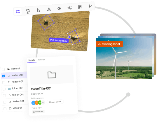
Human-in-the-loop aims to achieve what neither an algorithm nor a human can manage by themselves. Especially when training an algorithm, such as a computer vision model, it’s often helpful for human annotators or data scientists to provide feedback so the models gets a clearer understanding of what it’s being shown.
In most cases, human-in-the-loop processes can be deployed in either supervised or unsupervised learning.
In supervised learning, HITL model development, annotators or data scientists give a computer vision model labeled and annotated datasets.
HITL inputs then allow the model to map new classifications for unlabeled data, filling in the gaps at a far greater volume with higher accuracy than a human team could. Human-in-the-loop improves the accuracy and outputs from this process, ensuring a computer vision model learns faster and more successfully than without human intervention.
In unsupervised learning, a computer vision model is given largely unlabeled datasets, forcing them to learn how to structure and label the images or videos accordingly. HITL inputs are usually more extensive, falling under a deep learning exercise category.
The overall aim of human-in-the-loop inputs and feedback is to improve machine-learning outcomes.
With continuous human feedback and inputs, the idea is to make a machine learning or computer vision model smarter. With constant human help, the model produces better results, improving accuracy and identifying objects in images or videos more confidently.
In time, a model is trained more effectively, producing the results that project leaders need, thanks to human-in-the-loop feedback. This way, ML algorithms are more effectively trained, tested, tuned, and validated.
Although there are many advantages to human-in-the-loop systems, there are drawbacks too.
Using HITL processes can be slow and cumbersome, while AI-based systems can make mistakes, and so can humans. You might find that a human error goes unnoticed and then unintentionally negatively impacts a model's performance and outputs. Humans can’t work as quickly as computer vision models.
Hence the need to bring machines onboard to annotate datasets. However, once you’ve got people more deeply involved in the training process for machine learning models, it can take more time than it would if humans weren’t as involved.
One example is in the medical field, with healthcare-based image and video datasets. A 2018 Stanford study found that AI models performed better with human-in-the-loop inputs and feedback compared to when an AI model worked unsupervised or when human data scientists worked on the same datasets without automated AI-based support.
Humans and machines work better and produce better outcomes together. The medical sector is only one of many examples whereby human-in-the-loop ML models are used.
When undergoing quality control and assurance checks for critical vehicle or airplane components, an automated, AI-based system is useful; however, for peace of mind, having human oversight is essential.
Human-in-the-loop inputs are valuable whenever datasets are rare and a model is being fed. Such as a dataset containing a rare language or artifacts. ML models may not have enough data to draw from; human inputs are invaluable for training algorithmically-generated models.
With the right tools and platform, you can get a computer vision model to production faster.
Encord is one such platform, a collaborative, active learning suite of solutions for computer vision that can also be used for human-in-the-loop (HITL) processes.
With AI-assisted labeling, model training, and diagnostics, you can use Encord to provide the perfect ready-to-use platform for a HITL team, making accelerating computer vision model training and development easier. Collaborative active learning is at the core of what makes human-in-the-loop (HITL) processes so effective when training computer vision models. This is why it’s smart to have the right platform at your disposal to make this whole process smoother and more effective.
We also have Encord Active, an open-source computer vision toolkit, and an Annotator Training Module that will help teams when implementing human-in-the-loop iterative training processes.
At Encord, our active learning platform for computer vision is used by a wide range of sectors - including healthcare, manufacturing, utilities, and smart cities - to annotate human pose estimation videos and accelerate their computer vision model development.
Encord is a comprehensive AI-assisted platform for collaboratively annotating data, orchestrating active learning pipelines, fixing dataset errors, and diagnosing model errors & biases. Try it for free today.
Human-in-the-loop (HITL) is an iterative feedback process whereby a human (or team) interacts with an algorithmically-generated model. Providing ongoing feedback improves a model's predictive output ability, accuracy, and training outcomes.
Human-in-the-loop data annotation is the process of employing human annotators to label datasets. Naturally, this is widespread, with numerous AI-based tools helping to automate and accelerate the process.
However, HITL annotation takes human inputs to the next level, usually in the form of quality control or assurance feedback loops before and after datasets are fed into a computer vision model.
Human-in-the-loop optimization is simply another name for the process whereby human teams and data specialists provide continuous feedback to optimize and improve the outcomes and outputs from computer vision and other ML/AI-based models.
Active learning and human-in-the-loop are similar in many ways, and both play an important role in training computer vision and other algorithmically-generated models. Yes, they are compatible, and you can use both approaches in the same project.
However, the main difference is that the human-in-the-loop approach is broader, encompassing everything from active learning to labeling datasets and providing continuous feedback to the algorithmic model.
Almost any AI project can benefit from human-in-the-loop workflows, including computer vision, sentiment analysis, NLP, deep learning, machine learning, and numerous others. HITL teams are usually integral to either the data annotation part of the process or play more of a role in training an algorithmic model.
Join the Encord Developers community to discuss the latest in computer vision, machine learning, and data-centric AI
Join the communityRelated Blogs
Before OpenAI was a producer of the most scintillating boardroom corporate drama outside of an episode of Succession, it was the creator of the universally known AI application ChatGPT. On the eve of the one-year anniversary of its launch(a whirlwind year of progress, innovations, and twists), it is worth revisiting the state of AI post-ChatGPT with a view towards looking forward. A year ago, ChatGPT took the world by storm, smashing even OpenAI’s greatest expectations of adoption by becoming the world’s fastest-growing consumer app of all time. While the last year has been filled with a panoply of new models, hundreds of freshly minted startups, and gripping drama, it still very much feels like only the early days of the technology. As the cofounder of an AI company, and having been steeped in the ecosystem for years, the difference this last year has made has been nothing short of remarkable—not just in technological progress or academic research (although the strides here have been dizzying) —but more in unlocking the public imagination and discourse around AI. YCombinator, a leading barometer of the directionality of technological trends, has recently churned out batches where, for the first time, most companies are focused on AI. ChatGPT is now being used as a zinger in political debates. Once exotic terms like Retrieval Augmentation Generation are making their way into the vernacular of upper management in Fortune 500 companies. We have entered not a technological, but a societal change, where AI is palatable for mainstream digestion. So what’s next? Seeing the future is easy, if you know where to look in the present: technological progress does not move as a uniform front where adoption of innovation propagates equally across all facets of society. Instead, it moves like waves crashing the jagged rocks of a coastline, splashing chaotically forward, soaking some while leaving others dry. Observing where the water hits first lets you guess what happens when it splashes on others later. It takes one visit to San Francisco to notice the eerily empty vehicles traversing the city in a silent yet conspicuous manner to preview what the future looks like for municipalities around the world—a world with the elimination of Uber driver small talk. While making firm predictions in a space arguably moving forward faster than any other technological movement in history is a fool’s game, clear themes are emerging that are worth paying attention to by looking at the water spots of those closest to the waves. We are only one year into this “new normal,” and the future will have much more to bring along the following: Dive Into Complexity One of the most exciting aspects of artificial intelligence as a technology is that it falls into a category few technologies do: “unbounded potential.” Moore’s Law in the ‘60s gave a self-fulling prophecy of computational progress for Silicon Valley to follow. The steady march of development cycles has paved the way from room-sized machines with the power of a home calculator to all the marvellous wonders we take for granted in society today. Similar to computation, there are no limits in principle for the cognitive power of computers across the full range of human capabilities. This can stoke the terrors of a world-conquering AGI, but it also brings up a key principle worth considering: ever-increasing intellectual power. The AIs of today that are drawing boxes over cars and running segmentations over people will be considered crude antiquities in a few years. They are sub-component solutions used only as intermediate steps to tackle more advanced problems (such as diagnosing cancer, counting cars for parking tickets, etc). We must walk before we can run, but it is not difficult to imagine an ability to tackle harder and harder questions over time. In the future, AI will be able to handle problems of increasing complexity and nuance, ones that are currently limitations for existing systems. While ChatGPT and other equivalent LLMs of today are conversant (and hallucinatory) in wide-ranging topics, they still cannot handle niche topics with reliability. Companies, however, have already begun tailoring these models with specialized datasets and techniques to handle more domain-specific use cases. With improved training and prompting, the emergence of AI professionals - such as doctors, paralegals, and claims adjusters - is on the horizon. We’re also approaching an era where these specialized applications, like a FashionGPT trained on the latest trends, can provide personalized advice and recommendations according to individual preferences. We should expect a world where the complexity and nuance of problems, ones that are only available for particular domain experts of today, will be well within the scope of AI capabilities. Topics like advanced pathology, negotiating geopolitical situations, and company building will be problems within AI capacity. If the history of computers is any beacon, complexity is the direction forward. Multi-modality Right now, there are categorical boxes classifying different types of problems that AI systems can solve. We have “computer vision”, “NLP”, “reinforcement learning”, etc. We also have separations between “Predictive” and “Generative AI” (with a corresponding hype cycle accompanying the rise of the term). These categories are useful, but they are mostly in place because models can, by and large, solve one type of problem at a time. Whenever the categorizations are functions of technological limitations, you should not expect permanence; you should expect redefinitions. Humans are predictive and generative. You can ask me if a picture is of a cat or a dog, and I can give a pretty confident answer. But I can also draw a cat (albeit badly). Humans are also multi-modal. I can listen to the soundtrack of a movie and take in the sensory details of facial expressions, body language, and voice in both semantic content as well as tonal and volume variations. We are performing complex feats of sensor fusion across a spectrum of inputs, and we can perform rather complex inferences from these considerations. Given that we can do this adeptly, we shouldn’t expect any of these abilities to be outside the purview of sufficiently advanced models. The first inklings of this multi-modal direction are already upon us. ChatGPT has opened up to vision and can impressively discuss input images. Open-source models like LLaVA now reason over both text and vision. CLIP combines text and vision into a unified embedding structure and can be integrated with various types of applications. Other multimodal embedding agents are also becoming commonplace. {{gray_callout_start}} Check out my webinar with Frederik Hvilshøj, Lead ML Engineer at Encord, on “How to build Semantic Visual Search with ChatGPT & CLIP”. {{gray_callout_end}} While these multimodal models haven’t found use in many practical applications yet, it is only a matter of time before they are integrated into commonplace workflows and products. Tied to the point above on complexity, multimodal models will start to replace their narrower counterparts to solve more sophisticated problems. Today's models can, by and large, see, hear, read, plan, move, etc. The models of the future will do all of these simultaneously. The Many Faces of Alignment The future themes poised to gain prominence in AI not only encompass technological advancements but also their societal impacts. Among the onslaught of buzzy terms borne out of the conversations in San Francisco coffee shops, alignment has stood out among the rest as the catch-all for all the surrounding non-technical considerations of the broader implications of AI. According to ChatGPT: AI alignment refers to the process and goal of ensuring that artificial intelligence (AI) systems' goals, decisions, and behaviors are in harmony with human values and intentions. There are cascading conceptual circles of alignment dependent on the broadness of its application. As of now, the primary focus of laboratories and companies has been to align models to what is called a “loss function.” A loss function is a mathematical expression of how far away a model is from getting an answer “right.” At the end of the day, AI models are just very complicated functions, and all the surrounding infrastructure are very powerful functional optimization tool. A model behaving as it should as of now just means a function has been properly optimized to “having a low loss.” It begs the question of how you choose the right loss function in the first place. Is the loss function itself aligned with the broader goal of the researcher building it? Then there is the question: if the researcher is getting what they want, does the institution the researcher is sitting in get what it wants? The incentives of a research team might not necessarily be aligned with those of the company. There is the question of how all of this is aligned with the interests of the broader public, and so on. Dall-E’s interpretation of the main concentric circles of alignment The clear direction here is that infrastructure for disentangling multilevel alignment seems inevitable (and necessary). Research in “superalignment” by institutions such as OpenAI, before their board debacle, is getting heavy focus in the community. It will likely lead to tools and best practices to help calibrate AI to human intention even as AI becomes increasingly powerful. At the coarse-grained societal level, this is a broad regulation imposed by politicians who need help finding the Google toolbar. Broad-brushed regulations similar to what we see in the EU AI Act, are very likely to follow worldwide. Tech companies will get better at aligning models to their loss, researchers and alignment advocates at a loss to human goals, and regulators at the technology to the law. Regulation, self-regulation, and corrective mechanisms are bound to come—their effectiveness is still uncertain. The AI Internet A question in VC meetings all around the world is whether a small number of powerful foundation models will end up controlling all intelligence operations in the future or whether there will be a proliferation of smaller fine-tuned models floating around unmoored from centralized control. My guess is the answer is both. Clearly, centralized foundation models perform quite well on generalized questions and use cases, but it will be difficult for foundation model providers to get access to proprietary datasets housed in companies and institutions to solve finer-grained, domain-specific problems. Larger models are also constrained by their size and much more difficult to embed in edge devices for common workflows. For these issues, corporations will likely use alternatives to control their own fine-tuned models. Rather than having one model control everything, the future is likely to have many more AI models than today. The proliferation of AI models to come harkens back to the early proliferation of personal computing devices. The rise of the internet over the last 30 years has taught us a key lesson: things like to be connected. Intelligent models/agents will be no exception to this. AI agents, another buzz term on the rise, are according to ChatGPT: Systems or entities that act autonomously in an environment to achieve specific goals or perform certain tasks. We are seeing an uptake now on AI agents powered by various models tasked with specific responsibilities. Perhaps this will come down even to the individual level, where each person has their own personal AI completing the routine monotonous tasks for them on a daily basis. Whether this occurs or not, it is only a matter of time before these agents start to connect and communicate with each other. My scheduling assistant AI will need to talk to your scheduling assistant. AI will be social! My guess is a type of AI communication protocol will be one in which daisy-chaining models of different skills and occupations will exponentiate their individual usefulness. These communication protocols are still some ways from being established or formalized, but if the days of regular old computation mean much, they will not be far away. We are seeing the first Github repos showcasing orchestration systems of various models. While still crude, if you squint, you can see a world where this type of “AI internet” integrates into systems and workflows worldwide for everyday users. Paywalling The early internet provided a cornucopia of free content and usage powered by VC larges with the mandate of growth at all costs. It took a few years before the paywalls started, in news sites around the world, in walled-off premium features, and in jacked-up Uber rates. After proving the viability of a technology, the next logical step tends to be monetization. For AI, the days of open papers, datasets, and sharing in communities are numbered as the profit engine picks up. We have already seen this in the increasingly, almost comically, vague descriptions OpenAI releases about their models. By the time GPT-5 rolls around, the expected release won’t be much less guarded than OpenAI just admitting, “we used GPUs for this.” Even non-tech companies are realising that the data they possess has tremendous value and will be much more savvy before letting it loose. AI is still only a small portion of the economy at the moment, but its generality and unbounded potential stated above lead to the expectation that it can have absolutely enormous economic impact. Ironically, the value created by the early openness of technology will result in the end of technological sharing and a more closed mentality. The last generation of tech growth has been fueled by social media and “attention.” Any barriers to engagement, such as putting a credit card upfront, were discouraged, and the expectation that “everything is free” became commonplace in using many internet services. OpenAI, in contrast, rather than starting with a traditional ad-based approach for monetization, opened up a premium subscription service and is now charging hefty sums for tailored models for corporations. The value of AI technology in its own right obviates the middle step of funding through advertising. Data and intelligence will likely not come for free. As we shift from an attention economy to an intelligence economy, where automation becomes a core driver of growth, expect the credit cards to start coming out. Dall-E’s interpretation of the coming AI paywall paving the transition from an attention economy to an intelligence economy Expect the Unexpected As a usual mealy-mouthed hedge in any predictive article, the requisite disclaimer of the unimaginable items must be established. In this case, this is also a genuine belief. Even natural extrapolations of AI technology moving forward can leave us in heady disbelief of possible future states. Even much smaller questions, like if OpenAI itself will survive in a year, are extremely difficult to predict. If you asked someone 50 years ago about capturing some of the most magnificent imagery in the world, of items big or small, wonders of the world captured within a device in the palm of your hand and served in an endless scroll among other wonders, it would seem possible and yet inconceivable. Now, we are bored by seeing some of the world's most magnificent, spectacular images and events. Our demand for stimulating content is being overtaken by supply. Analogously, with AI, we might be in a world where scientific progress is accelerated beyond our wildest dreams, where we have more answers than questions, and where we cannot even process the set of answers available to us. Using AI, deep mathematical puzzles like the Riemann Hypothesis may be laid bare as a trivial exercise. Yet, the formulation of interesting questions might be bottlenecked by our own ability and appetite to answer them. A machine to push forward mathematical progress beyond our dreams might seem too much to imagine, but it’s only one of many surreal potential futures. If you let yourself daydream of infinite personal assistants, where you have movies of arbitrary storylines created on the fly for individual consumption, where you can have long and insightful conversations with a cast of AI friends, where most manual and cognitive work of the day has completely transformed, you start to realize that it will be difficult to precisely chart out where AI is going. There are of course both utopian and dystopian branches of these possibilities. The technology is agnostic to moral consequence; it is only the people using it and the responsibility they incur that can be considered in these calculations. The only thing to expect is that we won’t expect what’s coming. Conclusion Is ChatGPT the equivalent of AI what the iPhone moment of the app wave was in the early 2010s? Possibly—and probably why OpenAI ran a very Apple-like keynote before Sam Altman’s shocking dismissal and return. But what is clear is that once items have permeated into public consciousness, they cannot be revoked. People understand the potential now. Just 3 years ago a company struggling to raise a seed round had to compete for attention against crypto companies, payments processors, and fitness software. AI companies today are a hot ticket item and have huge expectations baked into this potential. It was only 9 months ago that I wrote about “bridging the gap” to production AI. Amidst all the frenzy around AI, it is difficult to forget that most models today are still only in the “POC” (Proof of Concept) state, not having proved sufficient value to be integrated with real-world applications. ChatGPT really showed us a world beyond just production, to “post-production” AI, where AI's broader societal interactions and implications become more of the story than the technological components that it’s made of. We are now at the dawn of the “Post-Production” era. Where this will go exactly is of course impossible to say. But if you look at the past, and at the present, the themes to watch for are: complexity, multi-modality, connectivity, alignment, commercialization, and surprise. I am certainly ready to be surprised.
November 29
Logistic regression is a statistical model used to predict the probability of a binary outcome based on independent variables. It is commonly used in machine learning and data analysis for classification tasks. Unlike linear regression, logistic regression uses a logistic function to model the relationship between independent variables and outcome probability. It has various applications, such as predicting customer purchasing likelihood, patient disease probability, online advertisement click probability, and the impact of social sciences on binary outcomes. Mastering logistic regression allows you to uncover valuable insights, optimize strategies, and enhance their ability to accurately classify and predict outcomes of interest. This article goes into more depth about logistic regression and gives a full look. The structure of the article is as follows: What is logistic regression? Data processing and implementation Model training and evaluation Challenges in logistic regression Real-world applications of Logistic Regression Implementation of logistic regression in Python Logistic regression: key takeaways Frequently Asked Questions (FAQs) What is Logistic Regression? Logistic regression is a statistical model used to predict the probability of a binary outcome based on one or more independent variables. Its primary purpose in machine learning is to classify data into different categories and understand the relationship between the independent and outcome variables. The fundamental difference between linear and logistic regression lies in the outcome variable. Linear regression is used when the outcome variable is continuous, while logistic regression is used when the outcome variable is binary or categorical. {{light_callout_start}} Linear regression shows the linear relationship between the independent (predictor) variable, i.e., the X-axis, and the dependent (output) variable, i.e., the Y-axis, called linear regression. If there is a single input variable (an independent variable), such linear regression is called simple linear regression. {{light_callout_end}} Types of logistic regressions Binary, ordinal, and multinomial systems are the three categories of logistic regressions. Let's quickly examine each of these in more detail. Binary regression Binary logistic regression is used when the outcome variable has only two categories, and the goal is to predict the probability of an observation belonging to one of the two categories based on the independent variables. Multinomial regression Multinomial logistic regression is used when the outcome variable has more than two categories that are not ordered. In this case, the logistic regression model will estimate the probabilities of an observation belonging to each category relative to a reference category based on the independent variables. Ordinal regression Ordinal logistic regression is used when the outcome variable has more than two categories that are ordered. Each type of logistic regression has its own specific assumptions and interpretation methods. Ordinal logistic regression is useful when the outcome variable's categories are arranged in a certain way. It lets you look at which independent variables affect the chance that an observation will be in a higher or lower category on the ordinal scale. Logistic Regression Curve Logistic Regression Equation The logistic regression equation The logistic regression equation is represented as: P(Y=1) = 1 / (1 + e^-(β0 + β1X1 + β2X2 + ... + βnXn)), where P(Y=1) is the probability of the outcome variable being 1, e is the base of the natural logarithm, β0 is the intercept, and β1 to βn are the coefficients for the independent variables X1 to Xn, respectively. The sigmoid function The sigmoid function, represented as: 1 / (1 + e^- (β0 + β1*X1 + β2*X2 + ... + βn*Xn)), is used in logistic regression to transform the linear combination of the independent variables into a probability. This sigmoid function ensures that the probability values predicted by the logistic regression equation always fall between 0 and 1. By adjusting the coefficients (β values) of the independent variables, logistic regression can estimate the impact of each variable on the probability of the outcome variable being 1. {{light_callout_start}} A sigmoid function is a bounded, differentiable, real function that is defined for all real input values and has a non-negative derivative at each point and exactly one inflection point. A sigmoid "function" and a sigmoid "curve" refer to the same object. {{light_callout_end}} Breakdown of the key components of the equation In logistic regression, the dependent variable is the binary outcome predicted or explained, represented as 0 and 1. Independent variables, or predictor variables, influence the dependent variable, either continuous or categorical. The coefficients, or β values, represent the strength and direction of the relationship between each independent variable, and the probability of the outcome variable is 1. Adjusting these coefficients can determine the impact of each independent variable on the predicted outcome. A larger coefficient indicates a stronger influence on the outcome variable. A simple example to illustrate the application of the equation: Let's consider a simple linear regression equation that predicts the sales of a product based on its price. The equation may look like this: Sales = 1000 - 50 * Price. In this equation, the coefficient of -50 indicates that for every unit increase in price, sales decrease by 50 units. So, if the price is $10, the predicted sales would be 1000 - 50 * 10 = 500 units. By manipulating the coefficient and the variables in the equation, we can analyze how different factors impact the sales of the product. If we increase the price to $15, the predicted sales would decrease to 1000 - 50 * 15 = 250 units. Conversely, if we decrease the price to $5, the predicted sales would increase to 1000 - 50 * 5 = 750 units. This equation provides us with a simple way to estimate the product's sales based on its price, allowing businesses to make informed pricing decisions. Assumptions of logistic regression In this section, you will learn the critical assumptions associated with logistic regression, such as linearity and independence. Understand Linear Regression Assumptions You will see why these assumptions are essential for the model's accuracy and reliability. Critical assumptions of logistic regression In logistic regression analysis, the assumptions of linearity and independence are important because they ensure that the relationships between the independent and dependent variables are consistent. This lets you make accurate predictions. Violating these assumptions can compromise the validity of the analysis and its usefulness in making informed pricing decisions, thus highlighting the importance of these assumptions. Assumptions impacting model accuracy and reliability in statistical analysis The model's accuracy and reliability are based on assumptions like linearity and independence. Linearity allows for accurate interpretation of independent variables' impact on log odds, while independence ensures unique information from each observation. The log odds, also known as the logit, are a mathematical transformation used in logistic regression to model the relationship between independent variables (predictors) and the probability of a binary outcome. Violations of these assumptions can introduce bias and confounding factors, leading to inaccurate results. Therefore, it's crucial to assess these assumptions during statistical analysis to ensure the validity and reliability of the results. Data Processing and Implementation In logistic regression, data processing plays an important role in ensuring the accuracy of the results with steps like handling missing values, dealing with outliers, and transforming variables if necessary. To ensure the analysis is reliable, using logistic regression also requires careful thought about several factors, such as model selection, goodness-of-fit tests, and validation techniques. Orange Data Mining - Preprocess Data preparation for logistic regression Data preprocessing for logistic regression involves several steps Firstly, handling missing values is crucial, as they can affect the model's accuracy. You can do this by removing the corresponding observations or assuming the missing values Next, dealing with outliers is important, as they can significantly impact the model's performance. Outliers can be detected using various statistical techniques and then either treated or removed depending on their relevance to the analysis. Additionally, transforming variables may be necessary to meet logistic regression assumptions. This can include applying logarithmic functions, square roots, or other mathematical transformations to the variables. Transforming variables can help improve the linearity and normality assumptions of logistic regressions. Finally, consider the multicollinearity issue, which occurs when independent variables in a logistic regression model are highly correlated. Addressing multicollinearity can be done through various techniques, such as removing one of the correlated variables or using dimension reduction methods like principal component analysis (PCA). Overall, handling missing values, outliers, transforming variables, and multicollinearity are all essential steps in preparing data for logistic regression analysis. Techniques for handling missing data and dealing with categorical variables Missing data can be addressed by removing observations with missing values or using imputation methods. Categorical variables must be transformed into numerical representations using one-hot encoding or dummy coding techniques. One-hot encoding creates binary columns for each category, while dummy coding creates multiple columns to avoid multicollinearity. These techniques help the model capture patterns and relationships within categorical variables, enabling more informed predictions. These methods ensure accurate interpretation and utilization of categorical information in the model. Significance of data scaling and normalization Data scaling and normalization are essential preprocessing steps in machine learning. Scaling transforms data to a specific range, ensuring all features contribute equally to the model's training process. On the other hand, normalization transforms data to a mean of 0 and a standard deviation of 1, bringing all variables to the same scale. This helps compare and analyze variables more accurately, reduces outliers, and improves the convergence of machine learning algorithms relying on normality. Overall, scaling and normalization are crucial for ensuring reliable and accurate results in machine learning models. Model Training and Evaluation Machine learning involves model training and evaluation. During training, the algorithm learns from input data to make predictions or classifications. Techniques like gradient descent or random search are used to optimize parameters. After training, the model is evaluated using separate data to assess its performance and generalization. Metrics like accuracy, precision, recall, and F1 score are calculated. The model is then deployed in real-world scenarios to make predictions. Regularization techniques can prevent overfitting, and cross-validation ensures robustness by testing the model on multiple subsets of the data. The goal is to develop a logistic regression model that generalizes well to new, unseen data. Process of training logistic regression models Training a logistic regression model involves several steps. Initially, the dataset is prepared, dividing it into training and validation/test sets. The model is then initialized with random coefficients and fitted to the training data. During training, the model iteratively adjusts these coefficients using an optimization algorithm (like gradient descent) to minimize the chosen cost function, often the binary cross-entropy. At each iteration, the algorithm evaluates the model's performance on the training data, updating the coefficients to improve predictions. Regularization techniques may be employed to prevent overfitting by penalizing complex models. This process continues until the model converges or reaches a predefined stopping criterion. Finally, the trained model's performance is assessed using a separate validation or test set to ensure it generalizes well to unseen data, providing reliable predictions for new observations. Cost functions and their role in model training In logistic regression, the cost function plays a crucial role in model training by quantifying the error between predicted probabilities and actual outcomes. The most common cost function used is the binary cross-entropy (or log loss) function. It measures the difference between predicted probabilities and true binary outcomes. The aim during training is to minimize this cost function by adjusting the model's parameters (coefficients) iteratively through techniques like gradient descent. As the model learns from the data, it seeks to find the parameter values that minimize the overall cost, leading to better predictions. The cost function guides the optimization process, steering the model towards better fitting the data and improving its ability to make accurate predictions. Evaluation metrics for logistic regression Precision: Precision evaluates the proportion of true positive predictions out of all positive predictions made by the model, indicating the model's ability to avoid false positives. Recall: Recall (or sensitivity) calculates the proportion of true positive predictions from all actual positives in the dataset, emphasizing the model's ability to identify all relevant instances. F1-score: The F1-score combines precision and recall into a single metric, balancing both metrics to provide a harmonic mean, ideal for imbalanced datasets. It assesses a model's accuracy by considering false positives and negatives in classification tasks. Accuracy: Accuracy measures the proportion of correctly classified predictions out of the total predictions made by the model, making it a simple and intuitive evaluation metric for overall model performance. These metrics help assess the efficiency and dependability of a logistic regression model for binary classification tasks, particularly in scenarios requiring high precision and recall, such as medical diagnoses or fraud detection. Challenges in Logistic Regression Logistic regression faces challenges such as multicollinearity, overfitting, and assuming a linear relationship between predictors and outcome log-odds. These issues can lead to unstable coefficient estimates, overfitting, and difficulty generalizing the model to new data. Additionally, the assumption may not always be true in practice. Common challenges faced in logistic regression Imbalanced datasets Imbalanced datasets lead to biased predictions towards the majority class and result in inaccurate evaluations for the minority class. This disparity in class representation hampers the model's ability to properly account for the less-represented group, affecting its overall predictive performance. Multicollinearity Multicollinearity arises from highly correlated predictor variables, making it difficult to determine the individual effects of each variable on the outcome. The strong interdependence among predictors further complicates the modeling process, impacting the reliability of the logistic regression analysis. {{light_callout_start}} Multicollinearity reduces the precision of the estimated coefficients, which weakens the statistical power of your regression model. You might be unable to trust the p-values to identify statistically significant independent variables. {{light_callout_end}} Overfitting Overfitting occurs when the model becomes overly complex and starts fitting noise in the data rather than capturing the underlying patterns. This complexity reduces the model's ability to generalize well to new data, resulting in a decrease in overall performance. Mitigation strategies and techniques Mitigation strategies, such as regularization and feature engineering, are crucial in addressing these challenges and improving the logistic regression model's predictive accuracy and reliability. Regularization techniques address overfitting in machine learning models. It involves adding a penalty term to the model's cost function, discouraging complex or extreme parameter values. This helps prevent the model from fitting the training data too closely and improves generalization. Polynomial terms raise predictor variables to higher powers, allowing for curved relationships between predictors and the target variable. This can capture more complex patterns that cannot be captured by a simple linear relationship. Interaction terms involve multiplying different predictor variables, allowing for the possibility that the relationship between predictors and the target variable differs based on the combination of predictor values. By including these non-linear terms, logistic regression can capture more nuanced and complex relationships, improving its predictive performance. Real-World Applications of Logistic Regression The real-world applications listed below highlight the versatility and potency of logistic regression in modeling complex relationships and making accurate predictions in various domains. Healthcare The healthcare industry has greatly benefited from logistic regression, which is used to predict the likelihood of a patient having a certain disease based on their medical history and demographic factors. It predicts patient readmissions based on age, medical history, and comorbidities. It is commonly employed in healthcare research to identify risk factors for various health conditions and inform public health interventions and policies. Banking and Finance Logistic regression is a statistical method used in banking and finance to predict loan defaults. It analyzes the relationship between income, credit score, and employment status variables. This helps institutions assess risk, make informed decisions, and develop strategies to mitigate losses. It also helps banks identify factors contributing to default risk and tailor marketing strategies. Remote Sensing In remote sensing, logistic regression is used to analyze satellite imagery to classify land cover types like forest, agriculture, urban areas, and water bodies. This information is crucial for urban planning, environmental monitoring, and natural resource management. It also helps predict vegetation indices, assess plant health, and aid irrigation and crop management decisions. {{gray_callout_start}} Explore inspiring customer stories ranging from cutting-edge startups to enterprise and international research organizations. Witness how tools and infrastructure are accelerating the development of groundbreaking AI applications. Dive into these inspiring narratives at Encord for a glimpse into the future of AI. {{gray_callout_end}} Implementation of Logistic Regression in Python Implementation of logistic regression in Python involves the following steps while using the sklearn library: Import necessary libraries, such as Numpy, Pandas, Matplotlib, Seaborn and Scikit-Learn Then, load and preprocess the dataset by handling missing values and encoding categorical variables. Next, split the data into training and testing sets. Train the logistic regression model using the fit() function on the training set. Make predictions on the testing set using the predict() function. Evaluate the model's accuracy by comparing the predicted values with the actual labels in the testing set. This can be done using evaluation metrics such as accuracy score, confusion matrix, and classification report. Additionally, the model can be fine-tuned by adjusting hyperparameters, such as regularization strength, through grid search or cross-validation techniques. The final step is to interpret and visualize the results to gain insights and make informed decisions based on the regression analysis. Simple Logistic Regression in Python Logistic regression predicts the probability of a binary outcome (0 or 1, yes or no, true or false) based on one or more input features. Here's a step-by-step explanation of implementing logistic regression in Python using the scikit-learn library: # Import all the necessary libraries import numpy as np import pandas as pd from sklearn.model_selection import train_test_split from sklearn.linear_model import LogisticRegression from sklearn.metrics import accuracy_score,confusion_matrix, classification_report import seaborn as sns import matplotlib.pyplot as plt # Load Titanic dataset from seaborn titanic_data = sns.load_dataset('titanic') titanic_data.drop('deck',axis=1,inplace=True) titanic_data.dropna(inplace=True) # Import label encoder from sklearn import preprocessing # label_encoder object knows how to understand word labels. label_encoder = preprocessing.LabelEncoder() # Encode labels in column 'sex' to convert Male as 0 and Female as 1. titanic_data['sex']= label_encoder.fit_transform(titanic_data['sex']) print(titanic_data.head()) # Select features and target variable X = titanic_data[['pclass', 'sex', 'age', 'sibsp', 'parch', 'fare']] y = titanic_data['survived'] # Split the dataset into training and test sets (e.g., 80-20 split) X_train, X_test, y_train, y_test = train_test_split(X, y, test_size=0.2, random_state=42) # Initialize and train the logistic regression model logistic_reg = LogisticRegression() logistic_reg.fit(X_train, y_train) # Make predictions on the test set predictions = logistic_reg.predict(X_test) # Calculate accuracy accuracy = accuracy_score(y_test, predictions) print("Accuracy:", accuracy) # Generate classification report print("Classification Report:") print(classification_report(y_test, predictions)) # Compute ROC curve and AUC from sklearn.metrics import roc_curve, auc fpr, tpr, thresholds = roc_curve(y_test, logistic_reg.predict_proba(X_test)[:, 1]) roc_auc = auc(fpr, tpr) # Plot ROC curve plt.figure(figsize=(8, 6)) plt.plot(fpr, tpr, color='blue', lw=2, label='ROC curve (AUC = %0.2f)' % roc_auc) plt.plot([0, 1], [0, 1], color='gray', linestyle='--') plt.xlabel('False Positive Rate') plt.ylabel('True Positive Rate') plt.title('Receiver Operating Characteristic (ROC) Curve') plt.legend(loc='lower right') plt.show() Outputs: Accuracy: 0.7902097902097902 ROC-AUC curve Interpretation Accuracy Our accuracy score is 0.79 (or 79.02%), which means that the model correctly predicted approximately 79% of the instances in the test dataset. Summary of classification report This classification report evaluates a model's performance in predicting survival outcomes (survived or not) based on various passenger attributes. For passengers who did not survive (class 0): The precision is 77%. When the model predicts a passenger didn't survive, it is accurate 77% of the time. For passengers who survived (class 1): The precision is 84%. When the model predicts a passenger survived, it is accurate 84% of the time. Recall For passengers who did not survive (class 0): The recall is 90%. The model correctly identifies 90% of all actual non-survivors. For passengers who survived (class 1): The recall is 65%. The model captures 65% of all actual survivors. F1-score For passengers who did not survive (class 0): The F1-score is 83%. For passengers who survived (class 1): The F1-score is 73%. There were 80 instances of passengers who did not survive and 63 instances of passengers who survived in the dataset. ROC Curve (Receiver Operating Characteristic) The ROC curve shows the trade-off between sensitivity (recall) and specificity (1 - FPR) at various thresholds. A curve closer to the top-left corner represents better performance. AUC (Area Under the Curve) Definition: AUC represents the area under the ROC curve. It quantifies the model's ability to distinguish between the positive and negative classes. A higher AUC value (closer to 1.0) indicates better discrimination; the model has better predictive performance. View the entire code here. Logistic Regression in Machine Learning {{gray_callout_start}} 🎯 Recommended: Accuracy vs. Precision vs. Recall in Machine Learning: What's the Difference? {{gray_callout_end}} Logistic Regression: Key Takeaways Logistic regression is a popular algorithm used for binary classification tasks. It estimates the probability of an event occurring based on input variables. It uses a sigmoid function to map the predicted probabilities to binary outcomes. Apply regularization to prevent overfitting and improve generalization. Logistic regression can be interpreted using coefficients, odds ratios, and p-values. Logistic regression is widely used in various fields, such as medicine, finance, and marketing, due to its simplicity and interpretability. The algorithm is particularly useful when dealing with imbalanced datasets, as it can handle the imbalance by adjusting the decision threshold. Logistic regression assumes a linear relationship between the input variables of the outcome, which can be a limitation in cases where the relationship is non-linear. Despite its limitations, logistic regression remains a powerful tool for understanding the relationship between input variables and the probability of an event occurring. {{Active_CTA}}
November 27
8 min
Imagine you are watching a football match. The sports analysts provide you with detailed statistics and expert opinions. At the same time, you also take into account the opinions of fellow enthusiasts who may have witnessed previous matches. This approach helps overcome the limitations of relying solely on one model and increases overall accuracy. Similarly, in ensemble learning, combining multiple models or algorithms can improve prediction accuracy. In both cases, the power of collective knowledge and multiple viewpoints is harnessed to make more informed and reliable predictions, overcoming the limitations of relying solely on one model. Let us take a deeper dive into what Ensemble Learning actually is. Ensemble learning is a machine learning technique that improves the performance of machine learning models by combining predictions from multiple models. By leveraging the strengths of diverse algorithms, ensemble methods aim to reduce both bias and variance, resulting in more reliable predictions. It also increases the model’s robustness to errors and uncertainties, especially in critical applications like healthcare or finance. Ensemble learning techniques like bagging, boosting, and stacking enhance performance and reliability, making them valuable for teams that want to build reliable ML systems. Ensemble Learning This article highlights the benefits of ensemble learning for reducing bias and improving predictive model accuracy. It highlights techniques to identify and manage uncertainties, leading to more reliable risk assessments, and provides guidance on applying ensemble learning to predictive modeling tasks. Here, we will address the following topics: Brief overview Ensemble learning techniques Benefits of ensemble learning Challenges and considerations Applications of ensemble learning Types of Ensemble Learning Ensemble learning differs from deep learning; the latter focuses on complex pattern recognition tasks through hierarchical feature learning. Ensemble techniques, such as bagging, boosting, stacking, and voting, address different aspects of model training to enhance prediction accuracy and robustness. These techniques aim to reduce bias and variance in individual models, and improve prediction accuracy by learning previous errors, ultimately leading to a consensus prediction that is often more reliable than any single model. {{light_callout_start}} The main challenge is not to obtain highly accurate base models but to obtain base models that make different kinds of errors. If ensembles are used for classification, high accuracies can be achieved if different base models misclassify different training examples, even if the base classifier accuracy is low. {{light_callout_end}} Bagging: Bootstrap aggregating Bootstrap aggregation, or bagging, is a technique that improves prediction accuracy by combining predictions from multiple models. It involves creating random subsets of data, training individual models on each subset, and combining their predictions. However, this only happens in regression tasks. For classification tasks, the majority vote is typically used. Bagging applies bootstrap sampling to obtain the data subsets for training the base learners. Random forest The Random Forest algorithm is a prime example of bagging. It creates an ensemble of decision trees trained on samples of datasets. Ensemble learning effectively handles complex features and captures nuanced patterns, resulting in more reliable predictions. However, it is also true that the interpretability of ensemble models may be compromised due to the combination of multiple decision trees. Ensemble models can provide more accurate predictions than individual decision trees, but understanding the reasoning behind each prediction becomes challenging. Bagging helps reduce overfitting by generating multiple subsets of the training data and training individual decision trees on each subset. It also helps reduce the impact of outliers or noisy data points by averaging the predictions of multiple decision trees. Ensemble Learning: Bagging & Boosting | Towards Data Science Boosting: Iterative learning Boosting is a technique in ensemble learning that converts a collection of weak learners into a strong one by focusing on the errors of previous iterations. The process involves incrementally increasing the weight of misclassified data points, so subsequent models focus more on difficult cases. The final model is created by combining these weak learners and prioritizing those that perform better. Gradient boosting Gradient Boosting (GB) trains each model to minimize the errors of previous models by training each new model on the remaining errors. This iterative process effectively handles numerical and categorical data and can outperform other machine learning algorithms, making it versatile for various applications. For example, you can apply Gradient Boosting in healthcare to predict disease likelihood accurately. Iteratively combining weak learners to build a strong learner can improve prediction accuracy, which could be valuable in providing insights for early intervention and personalized treatment plans based on demographic and medical factors such as age, gender, family history, and biomarkers. One potential challenge of gradient boosting in healthcare is its lack of interpretability. While it excels at accurately predicting disease likelihood, the complex nature of the algorithm makes it difficult to understand and interpret the underlying factors driving those predictions. This can pose challenges for healthcare professionals who must explain the reasoning behind a particular prediction or treatment recommendation to patients. However, efforts are being made to develop techniques that enhance the interpretability of GB models in healthcare, ensuring transparency and trust in their use for decision-making. {{light_callout_start}} Boosting is an ensemble method that seeks to change the training data to focus attention on examples that previous fit models on the training dataset have gotten wrong. {{light_callout_end}} Boosting in Machine Learning | Boosting and AdaBoost - GeeksforGeeks In the clinical literature, gradient boosting has been successfully used to predict, among other things, cardiovascular events, the development of sepsis, delirium, and hospital readmissions following lumbar laminectomy. {{medical_CTA_light}} Stacking: Meta-learning Stacking, or stacked generalization, is a model-ensembling technique that improves predictive performance by combining predictions from multiple models. It involves training a meta-model that uses the output of base-level models to make a final prediction. The meta-model, a linear regression, a neural network, or any other algorithm makes the final prediction. This technique leverages the collective knowledge of different models to generate more accurate and robust predictions. The meta-model can be trained using ensemble algorithms like linear regression, neural networks, or support vector machines. The final prediction is based on the meta-model's output. Overfitting occurs when a model becomes too closely fitted to the training data and performs poorly on new, unseen data. Stacking helps mitigate overfitting by combining multiple models with different strengths and weaknesses, thereby reducing the risk of relying too heavily on a single model’s biases or idiosyncrasies. For example, in financial forecasting, stacking combines models like regression, random forest, and gradient boosting to improve stock market predictions. This ensemble approach mitigates the individual biases in the model and allows easy incorporation of new models or the removal of underperforming ones, enhancing prediction performance over time. Voting Voting is a popular technique used in ensemble learning, where multiple models are combined to make predictions. Majority voting, or max voting, involves selecting the class label that receives the majority of votes from the individual models. On the other hand, weighted voting assigns different weights to each model's prediction and combines them to make a final decision. Both majority and weighted voting are methods of aggregating predictions from multiple models through a voting mechanism and strongly influence the final decision. Examples of algorithms that use voting in ensemble learning include random forests and gradient boosting (although it’s an additive model “weighted” addition). Random forest uses decision tree models trained on different data subsets. A majority vote determines the final forecast based on individual forecasts. For instance, in a random forest applied to credit scoring, each decision tree might decide whether an individual is a credit risk. The final credit risk classification is based on the majority vote of all trees in the forest. This process typically improves predictive performance by harnessing the collective decision-making power of multiple models. {{light_callout_start}} The application of either bagging or boosting requires the selection of a base learner algorithm first. For example, if one chooses a classification tree, then boosting and bagging would be a pool of trees with a size equal to the user’s preference. {{light_callout_end}} Benefits of Ensemble Learning Improved accuracy and stability Ensemble methods combine the strengths of individual models by leveraging their diverse perspectives on the data. Each model may excel in different aspects, such as capturing different patterns or handling specific types of noise. By combining their predictions through voting or weighted averaging, ensemble methods can improve overall accuracy by capturing a more comprehensive understanding of the data. This helps to mitigate the weaknesses and biases that may be present in any single model. Ensemble learning, which improves model accuracy in the classification model while lowering mean absolute error in the regression model, can make a stable model less prone to overfitting. Ensemble methods also have the advantage of handling large datasets efficiently, making them suitable for big data applications. Additionally, ensemble methods provide a way to incorporate diverse perspectives and expertise from multiple models, leading to more robust and reliable predictions. Robustness Ensemble learning enhances robustness by considering multiple models' opinions and making consensus-based predictions. This mitigates the impact of outliers or errors in a single model, ensuring more accurate results. Combining diverse models reduces the risk of biases or inaccuracies from individual models, enhancing the overall reliability and performance of the ensemble learning approach. However, combining multiple models can increase the computational complexity compared to using a single model. Furthermore, as ensemble models incorporate different algorithms or variations of the same algorithm, their interpretability may be somewhat compromised. Reducing overfitting Ensemble learning reduces overfitting by using random data subsets for training each model. Bagging introduces randomness and diversity, improving generalization performance. Boosting assigns higher weights to difficult-to-classify instances, focusing on challenging cases and improving accuracy. Iteratively adjusting weights allows boosting to learn from mistakes and build models sequentially, resulting in a strong ensemble capable of handling complex data patterns. Both approaches help improve generalization performance and accuracy in ensemble learning. Benefits of using Ensemble Learning on Land Use Data Challenges and Considerations in Ensemble Learning Model selection and weighting Selecting the right combination of models to include in the ensemble, determining the optimal weighting of each model's predictions, and managing the computational resources required to train and evaluate multiple models simultaneously. Additionally, ensemble learning may not always improve performance if the individual models are too similar or if the training data has a high degree of noise. The diversity of the models—in terms of algorithms, feature processing, and data perspectives—is vital to covering a broader spectrum of data patterns. Optimal weighting of each model's contribution, often based on performance metrics, is crucial to harnessing their collective predictive power. Therefore, careful consideration and experimentation are necessary to achieve the desired results with ensemble learning. Computational complexity Ensemble learning, involving multiple algorithms and feature sets, requires more computational resources than individual models. While parallel processing offers a solution, orchestrating an ensemble of models across multiple processors can introduce complexity in both implementation and maintenance. Also, more computation might not always lead to better performance, especially if the ensemble is not set up correctly or if the models amplify each other's errors in noisy datasets. Diversity and overfitting Ensemble learning requires diverse models to avoid bias and enhance accuracy. By incorporating different algorithms, feature sets, and training data, ensemble learning captures a wider range of patterns, reducing the risk of overfitting and ensuring the ensemble can handle various scenarios and make accurate predictions in different contexts. Strategies such as cross-validation help in evaluating the ensemble's consistency and reliability, ensuring the ensemble is robust against different data scenarios. Interpretability Ensemble learning models prioritize accuracy over interpretability, resulting in highly accurate predictions. However, this trade-off makes the ensemble model more challenging to interpret. Techniques like feature importance analysis and model introspection can help provide insights but may not fully demystify the predictions of complex ensembles. the factors contributing to ensemble models' decision-making, reducing the interpretability challenge. Real-World Applications of Ensemble Learning Healthcare Ensemble learning is utilized in healthcare for disease diagnosis and drug discovery. It combines predictions from multiple machine learning models trained on different features and algorithms, providing more accurate diagnoses. Ensemble methods also improve classification accuracy, especially in complex datasets or when models have complementary strengths and weaknesses. Ensemble classifiers like random forests are used in healthcare to achieve higher performance than individual models, enhancing the accuracy of these tasks. {{light_callout_start}} Here’s an article worth a read which talks of using AI & ML for detecting medical conditions. {{light_callout_end}} Agriculture Ensemble models combine multiple base models to reduce outliers and noise, resulting in more accurate predictions. This is particularly useful in sales forecasting, stock market analysis and weather prediction. In agriculture, ensemble learning can be applied to crop yield prediction. Combining the predictions of multiple models trained on different environmental factors, such as temperature, rainfall, and soil quality, ensemble methods can provide more accurate forecasts of crop yields. Ensemble learning techniques, such as stacking and bagging, improve performance and reliability. Take a peek at this wonderful article on Encord that shows how to accurately measure carbon content in forests and elevate carbon credits with Treeconomy. Insurance Insurance companies can also benefit from ensemble methods in assessing risk and determining premiums. By combining the predictions of multiple models trained on various factors such as demographics, historical data, and market trends, insurance companies can better understand potential risks and make more accurate predictions of claim probabilities. This can help them set appropriate premiums for their customers and ensure a fair and sustainable insurance business. Remote sensing Ensemble learning techniques, like isolation forests and SVM ensembles, detect data anomalies by comparing multiple models' outputs. They increase detection accuracy and reduce false positives, making them useful for identifying fraudulent transactions, network intrusions, or unexpected behavior. These methods can be applied in remote sensing by combining multiple models or algorithms, training on different data subsets, and combining predictions through majority voting or weighted averaging. One practical use of remote sensing can be seen in this article; it’s worth a read. Sports Ensemble learning in sports involves using multiple predictive models or algorithms to make more accurate predictions and decisions in various aspects of the sports industry. Common ensemble methods include model stacking and weighted averaging, which improve the accuracy and effectiveness of recommendation systems. By combining predictions from different models, such as machine learning algorithms or statistical models, ensemble learning helps sports teams, coaches, and analysts gain a better understanding of player performance, game outcomes, and strategic decision-making. This approach can also be applied to other sports areas, such as injury prediction, talent scouting, and fan engagement strategies. By the way, you may be surprised to hear that a sports analytics company found that their ML team was unable to iterate and create new features due to a slow internal annotation tool. As a result, the team turned to Encord, which allowed them to annotate quickly and create new ontologies. Read the full story here. {{light_callout_start}} Ensemble models' outcomes can easily be explained using explainable AI algorithms. Hence, ensemble learning is extensively used in applications where an explanation is necessary. {{light_callout_end}} Psuedocode for implementing ensemble learning models Pseudocode is a high-level and informal description of a computer program or algorithm that uses a mix of natural language and some programming language-like constructs. It's not tied to any specific programming language syntax. It is used to represent the logic or steps of an algorithm in a readable and understandable format, aiding in planning and designing algorithms before actual coding. How do you build an ensemble of models? Here's a pseudo-code to show you how: Algorithm: Ensemble Learning with Majority Voting Input: - Training dataset (X_train, y_train) - Test dataset (X_test) - List of base models (models[]) Output: - Ensemble predictions for the test dataset Procedure Ensemble_Learning: # Train individual base models for each model in models: model.fit(X_train, y_train) # Make predictions using individual models for each model in models: predictions[model] = model.predict(X_test) # Combine predictions using majority voting for each instance in X_test: for each model in models: combined_predictions[instance][model] = predictions[model][instance] # Determine the most frequent prediction among models for each instance ensemble_prediction[instance] = majority_vote(combined_predictions[instance]) return ensemble_prediction What does it do? It takes input of training data, test data, and a list of base models. The base models are trained on the training dataset. Predictions are made using each individual model on the test dataset. For each instance in the test data, the pseudocode uses a function majority_vote() (not explicitly defined here) to perform majority voting and determine the ensemble prediction based on the predictions of the base models. Here's an illustration with pseudocode on how to implement different ensemble models: Pseudo Code of Ensemble Learning Ensemble Learning: Key Takeaways Ensemble learning is a powerful technique that combines the predictions of multiple models to improve the accuracy and performance of recommendation systems. It can overcome the limitations of single models by considering the diverse preferences and tastes of different users. Ensemble techniques like bagging, boosting, and stacking enhance prediction accuracy and robustness by combining multiple models. Bagging reduces overfitting by averaging predictions from different data subsets. Boosting trains weak models sequentially, giving more weight to misclassified instances. Lastly, stacking combines predictions from multiple models, using another model to make the final prediction. These techniques demonstrate the power of combining multiple models to improve prediction accuracy and robustness. Combining multiple models reduces the impact of individual model errors and biases, leading to more reliable and consistent recommendations. Specific ensemble techniques like bagging, boosting, and stacking play a crucial role in achieving better results in ensemble learning.
November 24
8 min
Forget fragmented workflows, annotation tools, and Notebooks for building AI applications. Encord Data Engine accelerates every step of taking your model into production.