A Practical Guide to Active Learning for Computer Vision

Why do we need active learning?
Data is the fuel that powers modern deep learning models, and copious amounts of it are often required to train these neural networks to learn complex functions from high-dimensional data such as images and videos. When building new datasets or even repurposing existing data for a new task, the examples have to be annotated with labels in order to be used for training and testing.
However, this annotation process can sometimes be extensively time-consuming and expensive. Images and videos can often be scraped or even taken automatically, however labeling for tasks like segmentation and motion detection is laborious. Some domains, such as medical imaging, require domain knowledge from experts with limited accessibility.
Wouldn’t it be nice if we could pick out the 5% of examples most useful to our model, rather than labeling large swathes of redundant data points? This is the idea behind active learning.
What is active learning?
Active learning is an iterative process where a machine learning model is used to select the best examples to be labeled next. After annotation, the model is retrained on the new, larger dataset, then selects more data to be labeled until reaching a stopping criterion. This process is illustrated in the figure below.
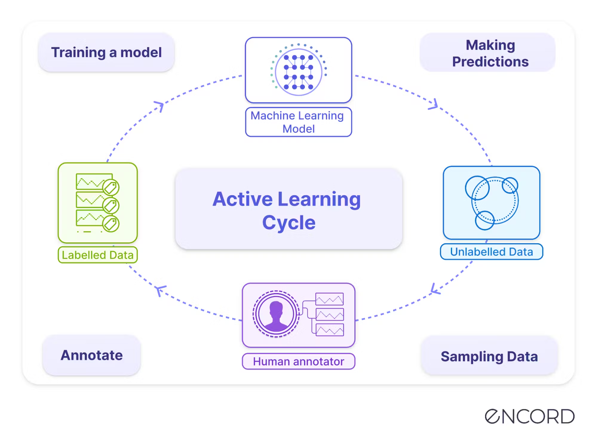
When examples are iteratively selected from an existing dataset, this corresponds to the pool-based active learning paradigm. We will focus on this problem setup as it reflects the overwhelming majority of real-world use cases.
Read more: Basic overview of active learning.
In this article, we will be going more in-depth into the following categories:
- Active learning methods
- Acquisition function
- How to design effective pipelines
- Common pitfalls to avoid when applying active learning to your own projects.
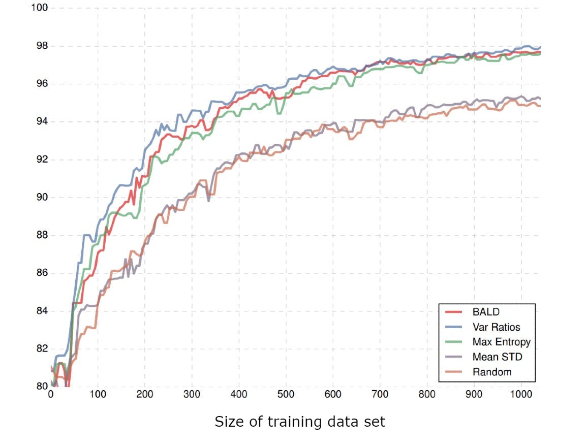
MNIST test accuracy from different active learning methods (source)
When to use active learning?
“Wow, reducing my annotation workload by a factor of 10x without sacrificing performance - sign me up!”. While active learning is an appealing idea, there are tradeoffs involved and it’s not the right move for every computer vision project.
As we said, the goal of active learning is to 1) identify gaps in your training data, 2) reduce the cost of the annotation process, and 3) maximize the performance of your model relative to the number of annotated training samples. Your first consideration should be whether or not it’s worth the cost tradeoff:
Annotation cost savings vs. Cost of implementation plus extra computation
Annotation costs: The comparison we need to make here will not be based on the cost of annotating the entire dataset, but the difference between annotating a sufficiently large enough random sample to train an accurate model vs the expected size of the sample chosen via active learning.
Cost of implementation: Building an active learning pipeline can be a particularly ops-heavy task. Data annotation is being coupled into the training process, so these two need to be tightly synchronized. Training and data selection for annotation should ideally be fully automated, with proper monitoring also put into place. The iterations will only be as efficient as their weakest link, requiring an annotation process capable of consistently fast turnaround times throughout sequential batches. Designing and implementing such a system requires MLOps skills and experience.
Computation costs: Active learning requires repeating the training process in each iteration, introducing a multiplier on the computation cost, which could be significant in cases involving very large, compute-heavy models, though usually this won’t be a limiting factor.
For many applications, this will still be worth the tradeoff. However, there are four other considerations you need to make before you begin:
- Biased data: Since we aren’t sampling randomly, the chosen training set will be biased by the model. This is done to maximize discriminative performance but can have major detrimental effects on things like density estimation, calibration, and explainability.
- Coupling of model and data: By performing active learning, you are coupling your annotation process with a specific model. The examples chosen for annotation by the particular selected model may not necessarily be the most useful for other models. Furthermore, since data tends to be more valuable than models and outlive models, you should ask yourself how much influence you want a particular model to have over the dataset. On the contrary, it may be reasonable to believe that particular chosen training subsets wouldn’t have large specific benefits between similar models.
- Difficulty of validation: In order to compare the performance of different active learning strategies, we need to annotate all examples chosen from all acquisition functions. This necessitates far more annotation cost than simply performing active learning, likely eliminating the desired cost savings. Even just comparing to a random sampling baseline could double the annotation cost (or more). Given sufficient training data at the current step, acquisition functions can be compared by simulating active learning within the current training dataset, however, this can add a noticeable amount of complexity to an already complex system. Often, different acquisition functions, models for data selection, and sizes of annotation batches are chosen upfront sans data.
- Brittleness: Finally, the performance of different acquisition functions can vary unpredictably among different models and tasks, and it’s not even uncommon for active learning to fail to outperform random sampling. Additionally, from 3, even just knowing how your active learning strategy compares to random sampling requires performing random sampling anyway.
“Ok, you’re really convincing me against this active learning thing - what are my alternatives?”
Active Learning Alternatives
Random Subsampling: So it’s not in the budget to annotate your entire dataset, but you still need training data for your model. The simplest approach here would be to annotate a random subset of your data. Random sampling has the major benefit of keeping your training set unbiased, which is expected by nearly all ML models anyway. In unbalanced data scenarios, you can also simultaneously balance your dataset via subsampling and get two birds with one stone here.
Clustering-based sampling: Another option is to choose a subsample with the goal of best representing the unlabeled dataset or maximizing diversity. For example, if you want to subsample k examples, you could apply the k-means algorithm (with k-clusters) to the hidden representations of your images from a pre-trained computer vision model. Then select one example from each resulting cluster. There are many alternative unsupervised and self-supervised methods here, such as VAE, SimCLR, or SCAN, but they are outside the scope of this article.
Manual Selection: In some instances, it may even make sense to curate a training subset manually. For tasks like segmentation, actually labeling the image takes far more work than determining whether it’s a challenging or interesting image to segment. For example, consider the case where we have an unbalanced dataset with certain rare objects or scenarios that we want to ensure make it into the training set. Those images could then be specifically selected manually (or automatically) for segmentation.
Should I use active learning?
Despite all of the potential issues and shortcomings outlined above, active learning has been demonstrated to be effective in scenarios across a wide variety of data modalities, domains, tasks, and models. For certain problems, there are few viable alternatives. For example, the field of autonomous driving often deals with enormous datasets of more than thousands of hours of video footage. Labeling each image for object detection or related tasks becomes very infeasible at scale. Additionally, driving video footage can be highly redundant. Sections containing unique conditions and precarious scenarios or difficult decision-making are rare. This presents a great opportunity for active learning to sort out relevant data for labeling.
For those of you still interested in applying this idea to your own problem, we’ll now give you an overview of common methods and how to build your own active learning pipeline.
Active Learning Methods
So, how do we actually choose which images to label? We want to select the examples that will be the most informative to our model, so a natural approach would be to score each example based on its predicted usefulness for training. Since we are labeling samples in batches, we could take the top k-scoring samples for annotation. This function that takes an unlabeled example and outputs its score is called an acquisition function. Here we give a brief overview of different acquisition functions and active learning strategies applicable to deep learning models. We will focus on the multiclass classification task, however, most of these approaches are easily modified to handle other computer vision tasks as well.
Uncertainty-based acquisition functions
The most common approach to scoring examples is uncertainty sampling, where we score data points based on the uncertainty of the model predictions. The assumption is that examples the model is confident about are likely to be more informative than examples for which our model is very confident about the label. Here are some common, straightforward acquisition functions for classification problems:
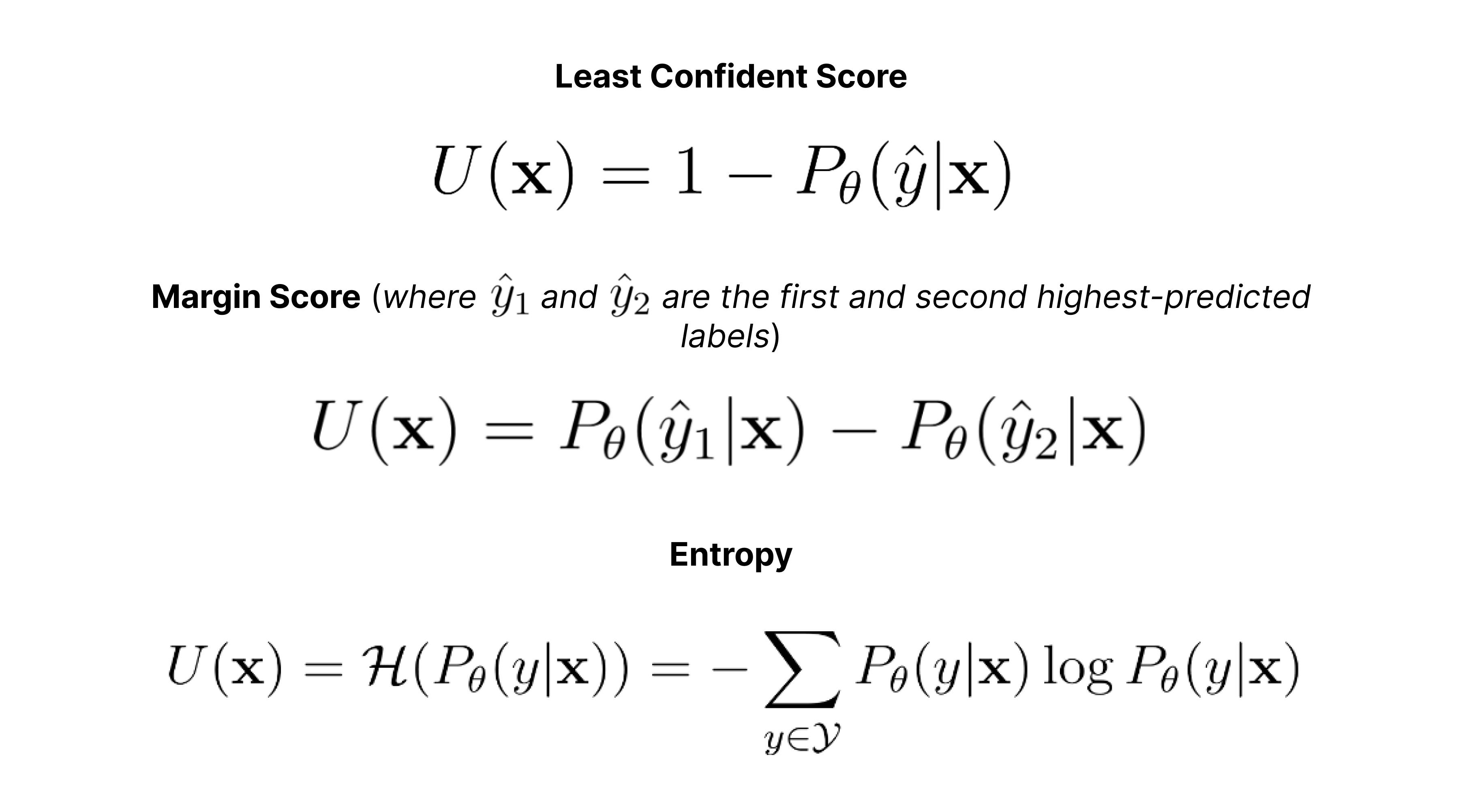
These acquisition functions are very simple and intuitive measures of uncertainty, however, they have one major drawback for our applications. Softmax outputs from deep networks are not calibrated and tend to be quite overconfident. For convolutional neural networks, small, seemingly meaningless perturbations in the input space can completely change predictions.
Query by Committee: Another popular approach to uncertainty estimation is using ensembles. With an ensemble of models, disagreement can be used as a measure of uncertainty. There are various ways to train ensembles and measure disagreement. Explicit ensembles of deep networks can perform quite well for active learning. However, this approach is usually very computationally expensive.
Bayesian Active Learning (Monte Carlo Dropout): When the topic of uncertainty estimation arises, one of your first thoughts is probably “Can we take a Bayesian approach?”. The most popular way to do this in deep active learning is Monte Carlo Dropout. Essentially, we can use dropout to simulate a deep gaussian process with Bernoulli weights. Then the posterior of our predictions is approximated by passing the input through our model multiple times with randomly applied dropout. Here is a pioneering paper on this technique.
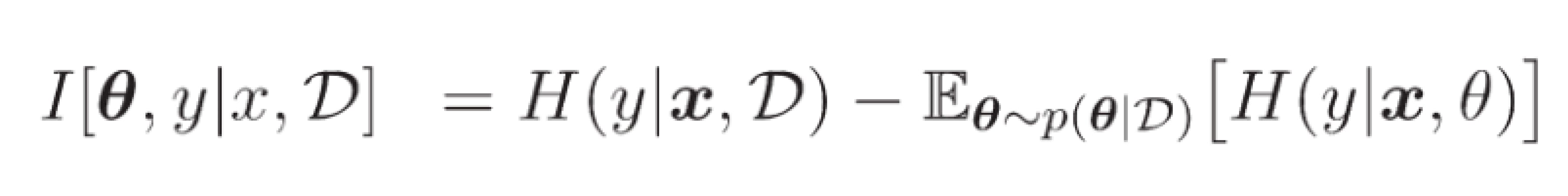
Bayesian Active Learning by Disagreement (BALD): On the subject of Bayesian active learning, Bayesian Active Learning through Disagreement (BALD), uses Monte Carlo Dropout to estimate the mutual information between the model’s output and its parameters:
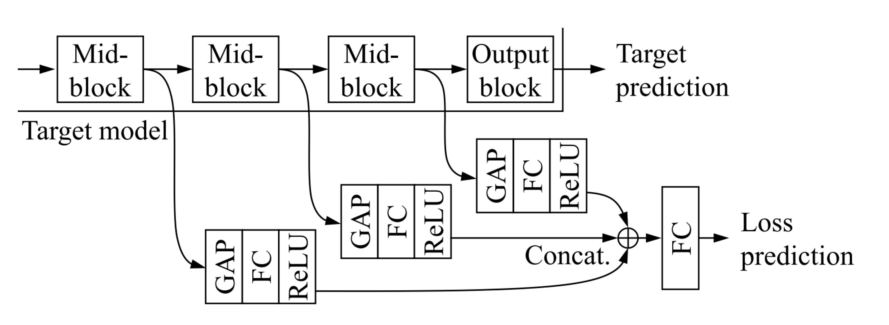
Loss Prediction: Loss prediction methods involve augmenting the neural network architecture with a module that outputs predictions of the loss for the given input. Unlabeled images with high predicted loss are then selected for labeling. It’s important to note that as the model is trained, loss on all examples will decrease. If a loss function like MSE is simply used to train the loss prediction head, then this loss will contribute less and less to the overall training loss as the model becomes more accurate. For this reason, a ranking-based loss is used to train the loss prediction head.
Diversity and Hybrid Acquisition Functions
So far we’ve looked at a handful of methods to score samples based on uncertainty. However, this approach has several potential issues:
- If the model is very uncertain about a particular class or type of example, then we can end up choosing an entire batch of very similar examples. If our batch size is large, then not only can this cause a lot of redundant labeling, but can leave us with an unbalanced and biased training set for the next iteration, especially early in the active learning process.
- Uncertainty-based methods are very prone to picking out outliers, examples with measurement errors, and other dirty data points that we don’t want to have overrepresented in our training set.
- These methods can result in quite biased training datasets in general.
An alternative approach is to select examples for labeling by diversity. Instead of greedily grabbing the most uncertain examples, we choose a set of examples that when added to the training set, best represents the underlying distribution. This results in less biased training datasets, and can usually be used with larger batch sizes and less iterations. We will also look at hybrid techniques where we prioritize uncertainty, but choose examples in a batch-aware manner to avoid issues like mode collapse within batches.
Core Sets: In computational geometry, a core set is a small set of points that best approximates a larger point set. In active learning, this corresponds to the strategy of selecting a small subset of data that best represents our larger unlabeled data set, such that a model trained on this subset is similar to a model trained after labeling all available data. This is done by choosing data points such that the distance between the latent feature representations of each sample in the unlabeled pool and its nearest neighbor in the labeled training set is minimized. Since this problem is NP-hard, a greedy algorithm is used.
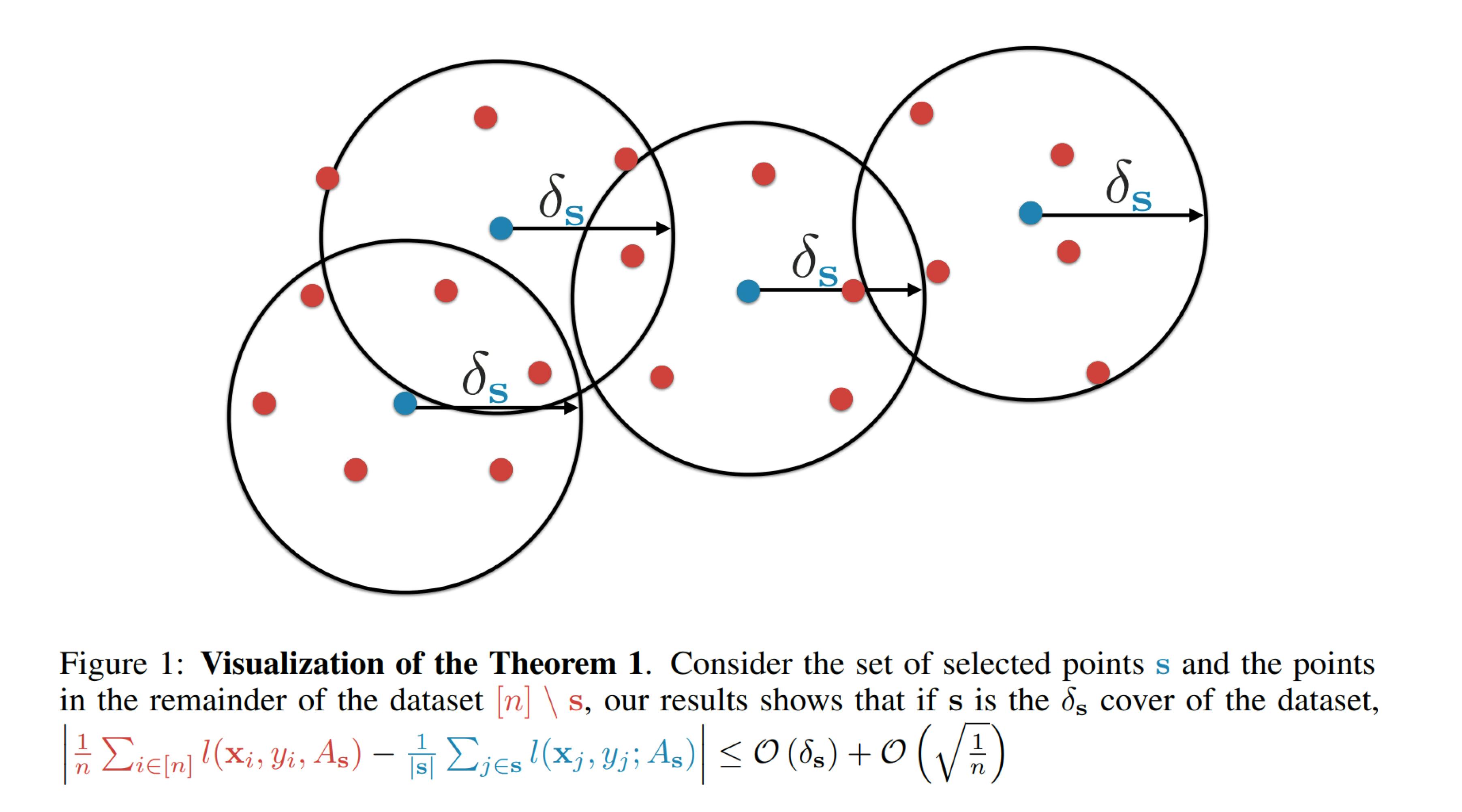
Core sets (source).
BatchBALD: BatchBALD is a batch-aware version of the BALD acquisition function where instead of maximizing the mutual information between a single model output and model parameters, we maximize the mutual information over the model outputs of all of the examples in the batch.
Bayesian Active Learning by Diverse Gradient Embeddings (BADGE): BADGE is another batch-aware method that, instead of using model outputs and hidden features, uses the gradient space to compare samples. Specifically, the gradient between the predicted class and the last layer of the network. The norm of this gradient is used to score the uncertainty of the samples (larger norm inputs have more effect during training and tend to be lower confidence). Then the gradient space is also used to create a diverse batch using kmeans++.
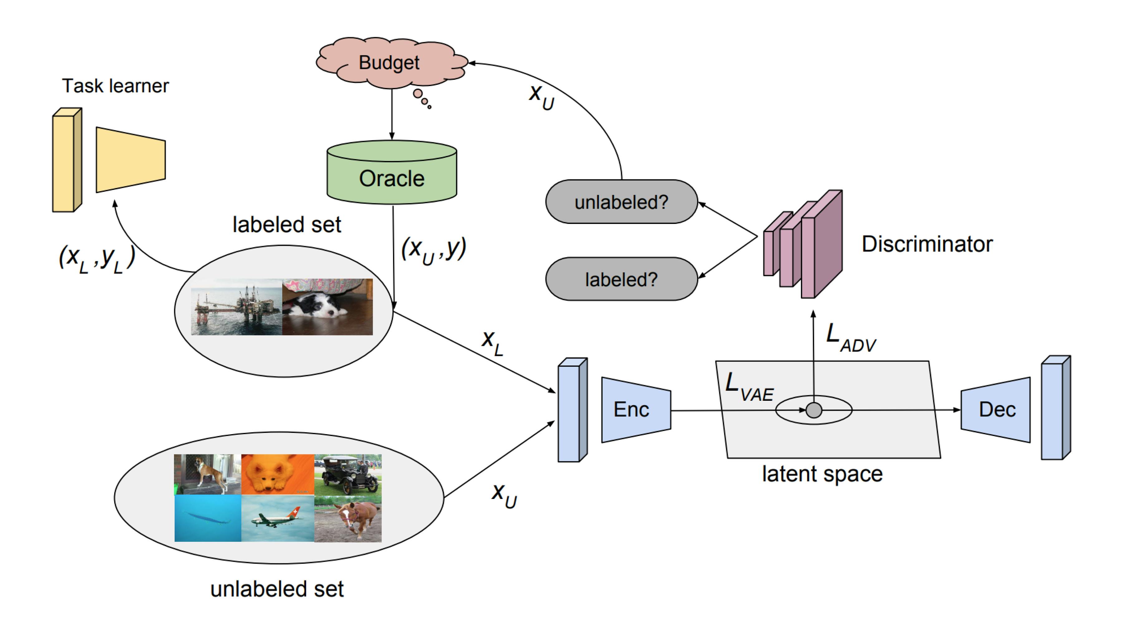
Adversarial Approaches: Variational Adversarial Active Learning (VAAL) uses a β-VAE to encode inputs into a latent space and a jointly-trained discriminator to distinguish between labeled and unlabeled examples. Examples that are most confidently predicted as unlabeled are chosen for labeling to maximize the diversity of the labeled set. Wasserstein Adversarial Active Learning (WAAL) further adopts the Wasserstein distance metric for distribution matching.
Which acquisition function should I use?
“Ok, I have this list of acquisition functions now, but which one is the best? How do I choose?”
This isn’t an easy question to answer and heavily depends on your problem, your data, your model, your labeling budget, your goals, etc. This choice can be crucial to your results and comparing multiple acquisition functions during the active learning process is not always feasible.
This isn’t a question for which we can just give you a good answer. Simple uncertainty measures like least confident score, margin score, entropy, and BALD make good first considerations. You can implement these with Monte Carlo Dropout. This survey paper compared a variety of different active learning techniques on a set of image classification problems and found WAAL and loss prediction to perform well on many datasets.
Tip! If you’d like to talk to an expert on the topic the Encord ML team can be found in the #help in our Active Learning Slack channel
Dataset Initialization
In the active learning paradigm our model selects examples to be labeled, however, to make these selections we need a model from which we can get useful representations or uncertainty metrics - a model that already “knows” something about our data.
This is typically accomplished by training an initial model on a random subset of the training data. Here, we want to use just enough data to get a model that can make our acquisition function useful to kickstart the active learning process.
Transfer learning with pre-trained models can further reduce the required size of the seed dataset and accelerate the whole process.
It’s also important to note that the test and validation datasets still need to be selected randomly and annotated in order to have unbiased performance estimates.
Stopping Criterion
The active learning procedure will need to be stopped at some point (otherwise we undermine ourselves and label all of the data anyway). Common stopping criteria include:
- Fixed annotation budget: Examples are labeled until a target number of labeled examples or spending is reached.
- Model performance target: Examples are labeled until a particular accuracy, precision, MSE, AUROC, or other performance metric is reached.
- Performance gain: Continue until the model performance gain falls under a specified threshold for one or more iterations.
- Manual review: You usually won’t be performing so many iterations that a manual review of performance is infeasible - just make sure that this is done asynchronously, so you don’t bleed efficiency by having annotators waiting for confirmation to proceed.
Model Selection
Once you have a final labeled dataset, model selection can be performed as usual. However, selecting a model for active learning is not a straightforward task. Often this is done primarily with domain knowledge rather than validating models with data. For example, we can search over architectures and hyperparameters using our initial seed training set. However, models that perform better in this limited data setting are not likely to be the best performing once we’ve labeled 10x as many examples.
Do we really want to use those models to select our data? No!
We should select data that optimizes the performance of our final model. So we want to use the type of model that we expect to perform best on our task in general.
Keep in mind that as our training set grows over each iteration, the size of our training epochs grows, and the hyperparameters and stopping criteria that maximize the performance of our model will change. Now, we could perform hyperparameter optimization each time we retrain the model, however, this strategy has the same issues that we discussed in the previous paragraph, and can dramatically increase the computation and time costs of the model fitting step. Yet again, the exact strategy you will use to handle this issue will depend on the details of your individual problem and situation.
Active Learning Pipelines
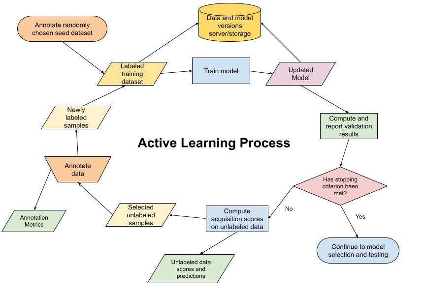
Example outline of an active learning pipeline
Efficiency
Ordinarily, data labeling is performed in one enormous batch. But with active learning, we split this process into multiple sequential batches of labeling. This introduces multiple possible efficiency leaks and potential slowdowns that need to be addressed, primarily:
Automation: Multiple cycles of labeling and model training can make the active learning process quite lengthy, so we want to make these iterations as efficient as possible. Firstly, we want there to be as little waiting downtime as possible. The only component of the active learning cycle that necessitates being performed manually is the actual annotation. All model training and data selection processes should be completely automated, for example, as DAG-based workflows. What we don’t want to happen is to have new labels sitting in a file somewhere waiting for someone to manually run a script to integrate them into the training dataset and begin fitting a new model.
Efficient Labeling: In the last point we discussed reducing downtime where all components are idling waiting for manual intervention. Time spent waiting for annotators should be minimized as well. Most data annotation services are set up to process large datasets as a single entity, not for fast turnaround times on smaller sequential batches. An inefficient labeling setup can dramatically slow down your system.
Labeling Batch Size: The size of the labeling “batches”, and the total number of iterations is a very important hyperparameter to consider. Larger batches and shorter iterations will reduce the time requirements of active learning. More frequent model updates can improve the quality of the data selection, however, batches should be large enough to sufficiently affect the model such that the selected data points are changed in each iteration.
Errors: It’s vital to have principled MLOps practices in place to ensure that active learning runs smoothly and bug-free. We’ll address this in the monitoring subsection.
Data Ops
Each active learning iteration introduces changes to both the data and model, requiring additional model and data versioning for reoganization. Additionally, data storage and transfer need to be handled appropriately. For example, you don’t want to be re-downloading all of the data to your model training server at each iteration. You only need the labeled examples and should be caching data appropriately.
Monitoring, Testing, and Debugging
The absolute last thing you want to happen when performing active learning is to realize that you’ve been sending the same examples to get re-labeled at every iteration for the past two weeks due to a bug. Proper testing is crucial - you should be checking the entire active learning workflow and training data platform thoroughly prior to large-scale implementation. Verifying the outputs of each component so that you can have confidence in your system before beginning labeling.
Monitoring is also an essential component of an active learning pipeline. It’s important to be able to thoroughly inspect a model’s performance at each iteration to quickly identify potential issues involving training, data selection, or labeling. Here are some ideas to get started:
Firstly, you need to monitor all of your usual model performance metrics after each training iteration. How is your model improving from increasing the size of the training set? If your model is not improving, then you have a problem. Some potential culprits are:
- Your labeling batch size is too small to make a noticeable difference.
- Your hyperparameter settings no longer suit your model due to the increased size of your training dataset.
- Your training dataset is already huge and you’ve saturated performance gains from more data.
- There is an issue/bug in your data selection process causing you to select bad examples.
Record the difference in acquisition function scores and rankings after the training step in each iteration. You are looking for:
- Scores for already labeled examples should be much lower than unlabeled examples on average. If not, you are selecting data points similar to already-labeled examples. If you’re using uncertainty sampling, this could mean that seeing the labels of examples is not improving your model's certainty (the uncertainty is coming from the problem itself rather than a shortcoming of your model).
- Does the set of highest-ranked data points change after training your model on newly-labeled samples? If not, updating the model is not changing the data selection. This could have the same potential causes outlined in 1.
Conclusion
In this article, we walked you through the steps to decide whether or not active learning is the right choice for your situation, presented an overview of important active learning methods, and enumerated important considerations for implementing active learning systems. Now you have the tools that you need to begin formulating active learning solutions for your own projects!
Want to get started with Active Learning?
“I want to start annotating” - Get a free trial of Encord here.
"I want to get started right away" - You can find Encord Active on Github here or try the quickstart Python command from our documentation.
"Can you show me an example first?" - Check out this Colab Notebook.
If you want to support the project you can help us out by giving a Star on GitHub ⭐
Want to stay updated?
- Follow us on Twitter and LinkedIn for more content on computer vision, training data, and active learning.
- Join the Slack community to chat and connect.
Frequently asked questions
Encord's active learning capabilities allow teams to automate the selection of data that is most valuable for model training, significantly reducing the time spent on manual data selection. This approach helps in identifying unperformant edge cases and improves overall model performance, making data a more valuable resource for AI development.
The new filtering system in Encord Active allows users to apply multiple filters more efficiently. By simply using the 'F' hotkey, users can quickly search for and apply filters like frame brightness or area without navigating through multiple menus, streamlining the workflow and enhancing usability.
Encord's active module allows teams to explore data at various levels, including frame, video, label, and prediction levels. This feature enables fine-grained filtering to identify edge cases and optimize model training by surfacing issues like brightness, darkness, and blurriness in the dataset.
Active learning in Encord's annotation process means that the platform intelligently selects the most informative samples for annotation, rather than requiring users to annotate all data. This approach increases efficiency by focusing on uncertain samples that will improve model performance.
Encord allows users to capture and visualize data effectively, enhancing it with internal metadata such as the source of the data and specific patient details. This capability enables better data curation and helps users slice and dice their data to improve their active learning processes.
Encord's active learning capabilities streamline the annotation process by leveraging automatic pipelines for identifying objects using vision libraries. This human-in-the-loop approach helps to efficiently manage outliers and enhances the overall quality of the training dataset.
Encord supports an active learning loop by allowing users to iteratively improve their models through continuous feedback and data refinement. This approach helps in identifying the most informative samples for labeling, thereby enhancing model accuracy and efficiency over time.
Encord Active is a feature that enables users to monitor and debug their annotation workflows. It helps in managing and curating data points while focusing on both the curation process and the annotation aspects, ensuring a seamless experience throughout the project lifecycle.
Yes, Encord supports active learning techniques by providing tools to help identify which images should be labeled next. This is an ongoing area of research within the platform, aimed at improving the efficiency of model training by selecting the most informative data points.
Encord incorporates active learning by turning labeled data into a project that continuously improves the model's performance. This process involves running cycles where the model learns from the labeled data, enhancing its accuracy and efficiency over time.