Logistic Regression: Definition, Use Cases, Implementation

Logistic regression is a statistical model used to predict the probability of a binary outcome based on independent variables. It is commonly used in machine learning and data analysis for classification tasks. Unlike linear regression, logistic regression uses a logistic function to model the relationship between independent variables and outcome probability. 

It has various applications, such as predicting customer purchasing likelihood, patient disease probability, online advertisement click probability, and the impact of social sciences on binary outcomes. Mastering logistic regression allows you to uncover valuable insights, optimize strategies, and enhance their ability to accurately classify and predict outcomes of interest.

This article goes into more depth about logistic regression and gives a full look. The structure of the article is as follows:

• What is logistic regression?
• Data processing and implementation 
• Model training and evaluation
• Challenges in logistic regression
• Real-world applications of Logistic Regression
• Implementation of logistic regression in Python
• Logistic regression: key takeaways
• Frequently Asked Questions (FAQs)

What is Logistic Regression?

Logistic regression is a statistical model used to predict the probability of a binary outcome based on one or more independent variables. Its primary purpose in machine learning is to classify data into different categories and understand the relationship between the independent and outcome variables. 

The fundamental difference between linear and logistic regression lies in the outcome variable. Linear regression is used when the outcome variable is continuous, while logistic regression is used when the outcome variable is binary or categorical. 

Linear regression shows the linear relationship between the independent (predictor) variable, i.e., the X-axis, and the dependent (output) variable, i.e., the Y-axis, called linear regression. If there is a single input variable (an independent variable), such linear regression is called simple linear regression.

Types of Logistic Regressions

Binary, ordinal, and multinomial systems are the three categories of logistic regressions. Let's quickly examine each of these in more detail.

Binary Regression

Binary logistic regression is used when the outcome variable has only two categories, and the goal is to predict the probability of an observation belonging to one of the two categories based on the independent variables.

Multinomial Regression

Multinomial logistic regression is used when the outcome variable has more than two categories that are not ordered. In this case, the logistic regression model will estimate the probabilities of an observation belonging to each category relative to a reference category based on the independent variables.

Ordinal Regression

Ordinal logistic regression is used when the outcome variable has more than two categories that are ordered. Each type of logistic regression has its own specific assumptions and interpretation methods. Ordinal logistic regression is useful when the outcome variable's categories are arranged in a certain way. It lets you look at which independent variables affect the chance that an observation will be in a higher or lower category on the ordinal scale.  

Logistic Regression Curve

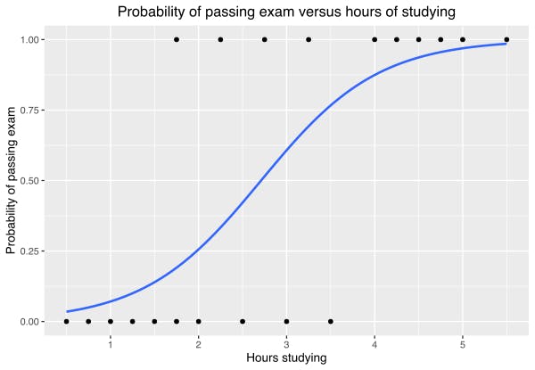
Logistic Regression Equation

The Logistic Regression Equation

The logistic regression equation is represented as:

P(Y=1) = 1 / (1 + e^-(β0 + β1X1 + β2X2 + ... + βnXn)),

where P(Y=1) is the probability of the outcome variable being 1, e is the base of the natural logarithm, β0 is the intercept, and β1 to βn are the coefficients for the independent variables X1 to Xn, respectively.

The Sigmoid Function

The sigmoid function, represented as:

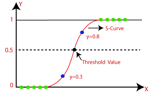
1 / (1 + e^- (β0 + β1*X1 + β2*X2 + ... + βn*Xn)), is used in logistic regression to transform the linear combination of the independent variables into a probability. This sigmoid function ensures that the probability values predicted by the logistic regression equation always fall between 0 and 1. 

By adjusting the coefficients (β values) of the independent variables, logistic regression can estimate the impact of each variable on the probability of the outcome variable being 1.

A sigmoid function is a bounded, differentiable, real function that is defined for all real input values and has a non-negative derivative at each point and exactly one inflection point. A sigmoid "function" and a sigmoid "curve" refer to the same object.

Breakdown of the Key Components of the Equation

In logistic regression, the dependent variable is the binary outcome predicted or explained, represented as 0 and 1. Independent variables, or predictor variables, influence the dependent variable, either continuous or categorical. 

The coefficients, or β values, represent the strength and direction of the relationship between each independent variable, and the probability of the outcome variable is 1. Adjusting these coefficients can determine the impact of each independent variable on the predicted outcome. A larger coefficient indicates a stronger influence on the outcome variable.
 

A simple example to illustrate the application of the equation will be a simple linear regression equation that predicts the sales of a product based on its price. The equation may look like this: 

Sales = 1000 - 50 * Price. In this equation, the coefficient of -50 indicates that for every unit increase in price, sales decrease by 50 units. So, if the price is $10, the predicted sales would be 1000 - 50 * 10 = 500 units. 

By manipulating the coefficient and the variables in the equation, we can analyze how different factors impact the sales of the product. If we increase the price to $15, the predicted sales would decrease to 1000 - 50 * 15 = 250 units. Conversely, if we decrease the price to $5, the predicted sales would increase to 1000 - 50 * 5 = 750 units. 

This equation provides us with a simple way to estimate the product's sales based on its price, allowing businesses to make informed pricing decisions.

Assumptions of Logistic Regression

In this section, you will learn the critical assumptions associated with logistic regression, such as linearity and independence.

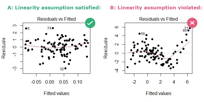
Understand Linear Regression Assumptions

You will see why these assumptions are essential for the model's accuracy and reliability.  

Critical Assumptions of Logistic Regression

In logistic regression analysis, the assumptions of linearity and independence are important because they ensure that the relationships between the independent and dependent variables are consistent. This lets you make accurate predictions. Violating these assumptions can compromise the validity of the analysis and its usefulness in making informed pricing decisions, thus highlighting the importance of these assumptions. 

Assumptions Impacting Model Accuracy and Reliability in Statistical Analysis

The model's accuracy and reliability are based on assumptions like linearity and independence. Linearity allows for accurate interpretation of independent variables' impact on log odds, while independence ensures unique information from each observation. The log odds, also known as the logit, are a mathematical transformation used in logistic regression to model the relationship between independent variables (predictors) and the probability of a binary outcome. Violations of these assumptions can introduce bias and confounding factors, leading to inaccurate results. Therefore, it's crucial to assess these assumptions during statistical analysis to ensure the validity and reliability of the results.

Data Processing and Implementation 

In logistic regression, data processing plays an important role in ensuring the accuracy of the results with steps like handling missing values, dealing with outliers, and transforming variables if necessary. 

To ensure the analysis is reliable, using logistic regression also requires careful thought about several factors, such as model selection, goodness-of-fit tests, and validation techniques.

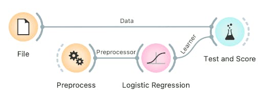
Orange Data Mining - Preprocess

Data Preparation for Logistic Regression

Data preprocessing for logistic regression involves several steps

• Firstly, handling missing values is crucial, as they can affect the model's accuracy. You can do this by removing the corresponding observations or assuming the missing values 
• Next, dealing with outliers is important, as they can significantly impact the model's performance. Outliers can be detected using various statistical techniques and then either treated or removed depending on their relevance to the analysis.
• Additionally, transforming variables may be necessary to meet logistic regression assumptions. This can include applying logarithmic functions, square roots, or other mathematical transformations to the variables. Transforming variables can help improve the linearity and normality assumptions of logistic regressions. 
• Finally, consider the multicollinearity issue, which occurs when independent variables in a logistic regression model are highly correlated. Addressing multicollinearity can be done through various techniques, such as removing one of the correlated variables or using dimension reduction methods like principal component analysis (PCA). 
• Overall, handling missing values, outliers, transforming variables, and multicollinearity are all essential steps in preparing data for logistic regression analysis.

Techniques for handling missing data and dealing with categorical variables

• Missing data can be addressed by removing observations with missing values or using imputation methods. 
• Categorical variables must be transformed into numerical representations using one-hot encoding or dummy coding techniques. One-hot encoding creates binary columns for each category, while dummy coding creates multiple columns to avoid multicollinearity. 
• These techniques help the model capture patterns and relationships within categorical variables, enabling more informed predictions. These methods ensure accurate interpretation and utilization of categorical information in the model.

Significance of data scaling and normalization

Data scaling and normalization are essential preprocessing steps in machine learning. Scaling transforms data to a specific range, ensuring all features contribute equally to the model's training process.

On the other hand, normalization transforms data to a mean of 0 and a standard deviation of 1, bringing all variables to the same scale. This helps compare and analyze variables more accurately, reduces outliers, and improves the convergence of machine learning algorithms relying on normality. Overall, scaling and normalization are crucial for ensuring reliable and accurate results in machine learning models.

Model Training and Evaluation

Machine learning involves model training and evaluation. During training, the algorithm learns from input data to make predictions or classifications. Techniques like gradient descent or random search are used to optimize parameters. 

After training, the model is evaluated using separate data to assess its performance and generalization. Metrics like accuracy, precision, recall, and F1 score are calculated. The model is then deployed in real-world scenarios to make predictions. Regularization techniques can prevent overfitting, and cross-validation ensures robustness by testing the model on multiple subsets of the data. The goal is to develop a logistic regression model that generalizes well to new, unseen data.

Process of Training Logistic Regression Models

Training a logistic regression model involves several steps. Initially, the dataset is prepared, dividing it into training and validation/test sets. The model is then initialized with random coefficients and fitted to the training data. During training, the model iteratively adjusts these coefficients using an optimization algorithm (like gradient descent) to minimize the chosen cost function, often the binary cross-entropy. 

At each iteration, the algorithm evaluates the model's performance on the training data, updating the coefficients to improve predictions. Regularization techniques may be employed to prevent overfitting by penalizing complex models. This process continues until the model converges or reaches a predefined stopping criterion. Finally, the trained model's performance is assessed using a separate validation or test set to ensure it generalizes well to unseen data, providing reliable predictions for new observations.

Cost Functions and their Role in Model Training

In logistic regression, the cost function plays a crucial role in model training by quantifying the error between predicted probabilities and actual outcomes. The most common cost function used is the binary cross-entropy (or log loss) function. It measures the difference between predicted probabilities and true binary outcomes. The aim during training is to minimize this cost function by adjusting the model's parameters (coefficients) iteratively through techniques like gradient descent. As the model learns from the data, it seeks to find the parameter values that minimize the overall cost, leading to better predictions. The cost function guides the optimization process, steering the model towards better fitting the data and improving its ability to make accurate predictions.

Evaluation Metrics for Logistic Regression

• Precision: Precision evaluates the proportion of true positive predictions out of all positive predictions made by the model, indicating the model's ability to avoid false positives.
• Recall: Recall (or sensitivity) calculates the proportion of true positive predictions from all actual positives in the dataset, emphasizing the model's ability to identify all relevant instances.
• F1-score: The F1-score combines precision and recall into a single metric, balancing both metrics to provide a harmonic mean, ideal for imbalanced datasets. It assesses a model's accuracy by considering false positives and negatives in classification tasks.
• Accuracy: Accuracy measures the proportion of correctly classified predictions out of the total predictions made by the model, making it a simple and intuitive evaluation metric for overall model performance.

These metrics help assess the efficiency and dependability of a logistic regression model for binary classification tasks, particularly in scenarios requiring high precision and recall, such as medical diagnoses or fraud detection.

Challenges in Logistic Regression

Logistic regression faces challenges such as multicollinearity, overfitting, and assuming a linear relationship between predictors and outcome log-odds. These issues can lead to unstable coefficient estimates, overfitting, and difficulty generalizing the model to new data. Additionally, the assumption may not always be true in practice. 

Common Challenges Faced in Logistic Regression

Imbalanced datasets

Imbalanced datasets lead to biased predictions towards the majority class and result in inaccurate evaluations for the minority class. This disparity in class representation hampers the model's ability to properly account for the less-represented group, affecting its overall predictive performance.

Multicollinearity

Multicollinearity arises from highly correlated predictor variables, making it difficult to determine the individual effects of each variable on the outcome. The strong interdependence among predictors further complicates the modeling process, impacting the reliability of the logistic regression analysis. 

Multicollinearity reduces the precision of the estimated coefficients, which weakens the statistical power of your regression model. You might be unable to trust the p-values to identify statistically significant independent variables.

Overfitting

Overfitting occurs when the model becomes overly complex and starts fitting noise in the data rather than capturing the underlying patterns. This complexity reduces the model's ability to generalize well to new data, resulting in a decrease in overall performance.

Mitigation Strategies and Techniques

Mitigation strategies, such as regularization and feature engineering, are crucial in addressing these challenges and improving the logistic regression model's predictive accuracy and reliability.

• Regularization techniques address overfitting in machine learning models. It involves adding a penalty term to the model's cost function, discouraging complex or extreme parameter values. This helps prevent the model from fitting the training data too closely and improves generalization. 
• Polynomial terms raise predictor variables to higher powers, allowing for curved relationships between predictors and the target variable. This can capture more complex patterns that cannot be captured by a simple linear relationship.
• Interaction terms involve multiplying different predictor variables, allowing for the possibility that the relationship between predictors and the target variable differs based on the combination of predictor values. By including these non-linear terms, logistic regression can capture more nuanced and complex relationships, improving its predictive performance.

Real-World Applications of Logistic Regression

The real-world applications listed below highlight the versatility and potency of logistic regression in modeling complex relationships and making accurate predictions in various domains. 

Healthcare

The healthcare industry has greatly benefited from logistic regression, which is used to predict the likelihood of a patient having a certain disease based on their medical history and demographic factors. It predicts patient readmissions based on age, medical history, and comorbidities. It is commonly employed in healthcare research to identify risk factors for various health conditions and inform public health interventions and policies. 

Banking and Finance

Logistic regression is a statistical method used in banking and finance to predict loan defaults. It analyzes the relationship between income, credit score, and employment status variables. This helps institutions assess risk, make informed decisions, and develop strategies to mitigate losses. It also helps banks identify factors contributing to default risk and tailor marketing strategies.  

Remote Sensing

In remote sensing, logistic regression is used to analyze satellite imagery to classify land cover types like forest, agriculture, urban areas, and water bodies. This information is crucial for urban planning, environmental monitoring, and natural resource management. It also helps predict vegetation indices, assess plant health, and aid irrigation and crop management decisions. 

Implementation of Logistic Regression in Python

Implementation of logistic regression in Python involves the following steps while using the sklearn library: 

1. Import necessary libraries, such as Numpy, Pandas, Matplotlib, Seaborn and Scikit-Learn
2. Then, load and preprocess the dataset by handling missing values and encoding categorical variables. 
3. Next, split the data into training and testing sets. 
4. Train the logistic regression model using the fit() function on the training set. 
5. Make predictions on the testing set using the predict() function. 
6. Evaluate the model's accuracy by comparing the predicted values with the actual labels in the testing set. This can be done using evaluation metrics such as accuracy score, confusion matrix, and classification report.
7. Additionally, the model can be fine-tuned by adjusting hyperparameters, such as regularization strength, through grid search or cross-validation techniques. 
8. The final step is to interpret and visualize the results to gain insights and make informed decisions based on the regression analysis.

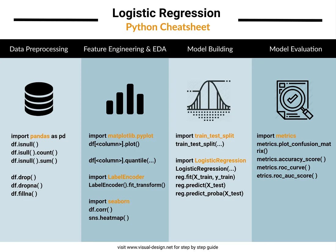
Simple Logistic Regression in Python

Logistic regression predicts the probability of a binary outcome (0 or 1, yes or no, true or false) based on one or more input features. 

Here's a step-by-step explanation of implementing logistic regression in Python using the scikit-learn library:

# Import all the necessary libraries
import numpy as np
import pandas as pd
from sklearn.model_selection import train_test_split
from sklearn.linear_model import LogisticRegression
from sklearn.metrics import accuracy_score,confusion_matrix, classification_report
import seaborn as sns
import matplotlib.pyplot as plt

# Load Titanic dataset from seaborn
titanic_data = sns.load_dataset('titanic')
titanic_data.drop('deck',axis=1,inplace=True)
titanic_data.dropna(inplace=True)

# Import label encoder
from sklearn import preprocessing

# label_encoder object knows how to understand word labels.
label_encoder = preprocessing.LabelEncoder()

# Encode labels in column 'sex' to convert Male as 0 and Female as 1.
titanic_data['sex']= label_encoder.fit_transform(titanic_data['sex'])
print(titanic_data.head())

# Select features and target variable
X = titanic_data[['pclass', 'sex', 'age', 'sibsp', 'parch', 'fare']]
y = titanic_data['survived']

# Split the dataset into training and test sets (e.g., 80-20 split)
X_train, X_test, y_train, y_test = train_test_split(X, y, test_size=0.2, random_state=42)

# Initialize and train the logistic regression model
logistic_reg = LogisticRegression()
logistic_reg.fit(X_train, y_train)

# Make predictions on the test set
predictions = logistic_reg.predict(X_test)

# Calculate accuracy
accuracy = accuracy_score(y_test, predictions)
print("Accuracy:", accuracy)

# Generate classification report
print("Classification Report:")
print(classification_report(y_test, predictions))

# Compute ROC curve and AUC
from sklearn.metrics import roc_curve, auc
fpr, tpr, thresholds = roc_curve(y_test, logistic_reg.predict_proba(X_test)[:, 1])
roc_auc = auc(fpr, tpr)

# Plot ROC curve
plt.figure(figsize=(8, 6))
plt.plot(fpr, tpr, color='blue', lw=2, label='ROC curve (AUC = %0.2f)' % roc_auc)
plt.plot([0, 1], [0, 1], color='gray', linestyle='--')
plt.xlabel('False Positive Rate')
plt.ylabel('True Positive Rate')
plt.title('Receiver Operating Characteristic (ROC) Curve')
plt.legend(loc='lower right')
plt.show()

Output:

Accuracy: 0.7902097902097902

ROC-AUC curve

Interpretation

Accuracy

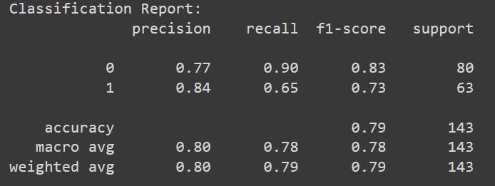
Our accuracy score is 0.79 (or 79.02%), which means that the model correctly predicted approximately 79% of the instances in the test dataset.

Summary of classification report

• This classification report evaluates a model's performance in predicting survival outcomes (survived or not) based on various passenger attributes.
• For passengers who did not survive (class 0): The precision is 77%. When the model predicts a passenger didn't survive, it is accurate 77% of the time.
• For passengers who survived (class 1): The precision is 84%. When the model predicts a passenger survived, it is accurate 84% of the time.

Recall

• For passengers who did not survive (class 0): The recall is 90%. The model correctly identifies 90% of all actual non-survivors.
• For passengers who survived (class 1): The recall is 65%. The model captures 65% of all actual survivors.

F1-score

• For passengers who did not survive (class 0): The F1-score is 83%.
• For passengers who survived (class 1): The F1-score is 73%.
• There were 80 instances of passengers who did not survive and 63 instances of passengers who survived in the dataset.

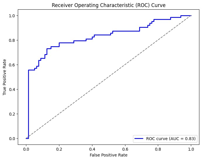
ROC Curve (Receiver Operating Characteristic)

• The ROC curve shows the trade-off between sensitivity (recall) and specificity (1 - FPR) at various thresholds. A curve closer to the top-left corner represents better performance.

AUC (Area Under the Curve)

• Definition: AUC represents the area under the ROC curve. It quantifies the model's ability to distinguish between the positive and negative classes.
• A higher AUC value (closer to 1.0) indicates better discrimination; the model has better predictive performance.

View the entire code here.

Logistic Regression in Machine Learning

Logistic Regression: Key Takeaways

• Logistic regression is a popular algorithm used for binary classification tasks. 
• It estimates the probability of an event occurring based on input variables.
• It uses a sigmoid function to map the predicted probabilities to binary outcomes.
• Apply regularization to prevent overfitting and improve generalization.
• Logistic regression can be interpreted using coefficients, odds ratios, and p-values. 
• Logistic regression is widely used in various fields, such as medicine, finance, and marketing, due to its simplicity and interpretability.
• The algorithm is particularly useful when dealing with imbalanced datasets, as it can handle the imbalance by adjusting the decision threshold.
• Logistic regression assumes a linear relationship between the input variables of the outcome, which can be a limitation in cases where the relationship is non-linear.
• Despite its limitations, logistic regression remains a powerful tool for understanding the relationship between input variables and the probability of an event occurring.
  

Evaluate your models and build active learning pipelines with Encord

Try Encord today