The Complete Guide to Data Annotation [2026 Review]

Co-Founder & CEO at Encord
TL;DR: Data annotation is how raw images and videos become training fuel for ML and computer vision models. Annotators label what's in each frame, such as tumours in a DICOM scan, erosion patterns in SAR satellite imagery, defects on a production line, etc., so models can learn to recognise the same patterns on their own. This guide walks through annotation types, real-world use cases across healthcare, manufacturing, smart cities, and defense, and the practical mechanics of labelling images and video.
Every computer vision model you've ever interacted with, the one flagging anomalies on a radiologist's screen, spotting cracks in a wind turbine, or guiding a warehouse robot around a pallet, started with someone drawing boxes, masks, or keypoints on thousands of images. That work is data annotation, and it's the bottleneck of almost every CV and ML project. The data format varies by domain; medical teams work with DICOM and NIfTI, geospatial teams handle Synthetic Aperture Radar, and ADAS teams deal with multi-camera video and LiDAR. The principle stays the same; labels have to match what the model is meant to learn before it ever sees production. Below, we'll break down the main annotation types, where they're used, and how to actually do it well.
What is Data Annotation?
Data annotation is the process of labeling raw data, images, video, text, audio, or sensor data, with the information a machine learning model needs to learn from it. A model can't infer on its own that a shape in a photo is a pedestrian or that a sentence expresses frustration; annotation is the step where a human (or a human-supervised system) supplies that ground truth.
The scope has grown well beyond images and video. Text annotation underpins everything from search relevance to chatbot intent recognition. Audio annotation trains transcription and voice assistant models. And the rise of large language models has added an entirely new category: RLHF and preference annotation, where humans rank model outputs rather than label raw content.
This guide covers all of it, with the deepest detail on the modality where Encord is used most: multimodal and physical AI data (video, 3D, sensor fusion) for robotics, autonomous systems, and healthcare.
The global market for labeled training data is expanding fast, tracking the same trajectory as foundation model and robotics investment. The data annotation tools market is valued at $2.1 billion in 2026, projected to reach $5.3 billion by 2030 at a CAGR of 26.3% (Grand View Research, 2026). Zoom out to the broader data collection and labeling market, which includes services alongside tools, and the numbers get bigger: $3.77 billion in 2024, growing to $17.1 billion by 2030 at a CAGR of 28.4%, with image and video annotation already commanding over 40% share of that market (Grand View Research, 2025). That last figure matters for teams building physical AI and robotics systems specifically, since visual data is where the bulk of annotation spend and complexity is concentrated. As AI models move from text-based tasks into multimodal and embodied use cases, demand for accurate, structured, and domain-specific labeled data is only going to climb.
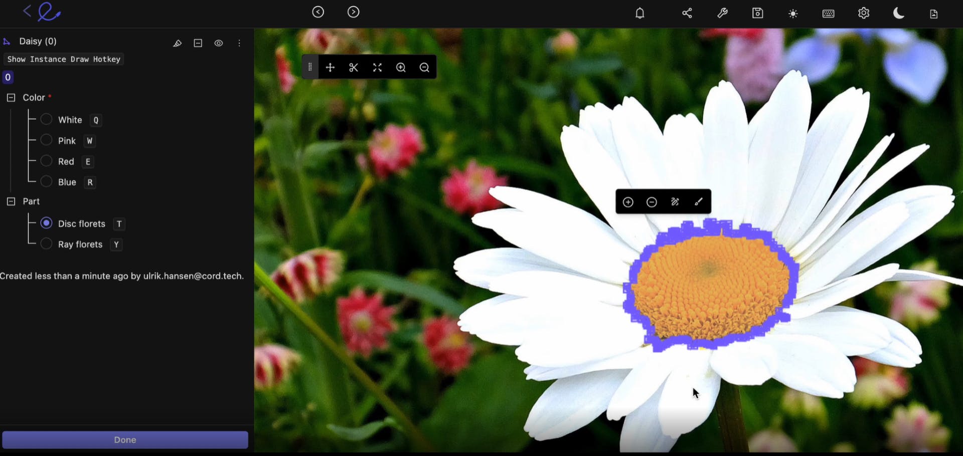
Image segementation in Encord
How AI-assisted labeling speeds up annotation
Manual annotation doesn't scale on its own. A single autonomous vehicle dataset can require millions of labeled frames; a robotics dataset built from multi-camera rigs multiplies that further. AI-assisted labeling (sometimes called model-assisted labeling, MAL) uses a model, often one already partially trained on your data, to pre-label a dataset, so human annotators are correcting and confirming rather than drawing from scratch.
This doesn't remove the human from the loop. In every serious annotation pipeline, a person still defines the ontology, corrects the model's early mistakes, and reviews output for quality. What changes is where their time goes: less time on repetitive, well-understood cases, more time on genuine edge cases and QA. Teams typically introduce AI assistance in stages, starting with the easiest object classes, then expanding assistance as the model's precision on that class clears a quality threshold.
Manual vs. platform-assisted vs. AI-assisted annotation
| Factor | Manual | Platform-assisted | AI-assisted (Encord) |
| Speed at scale | Slow, linear with headcount | Faster, workflow-managed | Fastest, model-in-the-loop pre-labeling |
| Consistency | Varies by annotator | Improved via guidelines and review | Consensus scoring and inter-annotator agreement tracking |
| Modality support | Single modality typical | Often single or dual modality | Image, video, audio, text, DICOM, 3D/LiDAR in one platform |
| Quality control | Manual spot-checks | Structured QA workflows | Automated quality metrics plus human review loop |
| Quality control | Manual spot-checks | Structured QA workflows | Automated quality metrics plus human review loop |
| Cost driver | Headcount hours | Platform fee plus headcount | Platform fee, reduced headcount need |
What Are The Different Types of Data Annotation?
There are numerous different ways to approach data annotation different data types
Image and video annotation techniques
Before going into more detail on the different types of image and video annotation projects, we also need to consider image classification and the difference between that and annotation. Although classification and annotation are both used to organize and label images to create high-quality image data, the processes and applications involved are somewhat different.
Classification is the act of automatically classifying objects in images or videos based on the groupings of pixels. Classification can either be “supervised”, with the support of human annotators, or “unsupervised”, done almost entirely with image labeling tools.
Alongside classification, there is a range of approaches that can be used to annotate images and videos:
- Multi-Object Tracking (MOT) in video annotation for computer vision models, is a way to track multiple objects from frame to frame in videos once an object has been labeled. For example, it could be a series of cars moving from one frame to the next in a video dataset. Using MOT, an automated annotation feature, it’s easier to keep track of objects, even if they change speed, direction, or light levels change.
- Interpolation in automated video annotation is a way of filling in the gaps between keyframes in a video. Once labels and annotations have been applied at the start and end of a series of videos, interpolation is an automation tool that applies those labels throughout the rest of the video(s) to accelerate the process.
- Auto Object Segmentation and detection is another type of automated data annotation tool. You can use this for recognizing and localizing objects in images or videos with vector labels. Types of segmentation include instance segmentation and semantic segmentation.
- Model-assisted labeling (MAL) or AI-assisted labeling (AAL) is another way of saying that automated tools are used in the labeling process. It’s far more complex than applying ML to spreadsheets or other data sources, as the content itself is either moving, multi-layered (in the case of various medical imaging datasets) or involves numerous complex objects, increasing the volume of labels and annotations required.
- Human Pose Estimation (HPE) and tracking is another automation tool that improves human pose and movement tracking in videos for computer vision models.
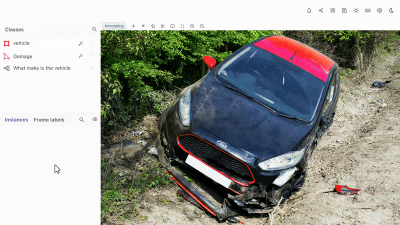
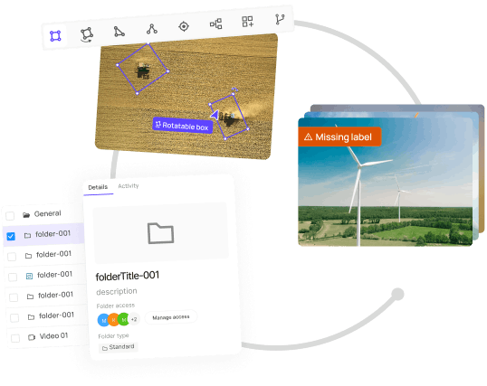
- Bounding Boxes: A way to draw a box around an object in an image or video, and then label that object so that automation tools can track it and similar objects throughout a dataset.
- Polygons and Polylines: These are ways of drawing lines and labeling either static or moving objects within videos and images, such as a road or railway line.
- Keypoints and Primitives (aka skeleton templates): Keypoints are useful for pinpointing and identifying features of countless shapes and objects, such as the human face. Whereas, primitives, also known as skeleton templates are for specialized annotations to templatize specific shapes, e.g. 3D cuboids, or the human body.
Text and NLP annotation
Text annotation adds structure to unstructured language so a model can extract meaning from it. The core techniques:
- Named entity recognition (NER): tagging spans of text as people, organizations, dates, or domain-specific entities. This is foundational to search, document processing, and information extraction.
- Sentiment annotation: labeling text as positive, negative, or neutral, used to train models that route support tickets or gauge product feedback.
- Intent annotation: labeling what a user is trying to accomplish with a piece of text, the backbone of chatbot and voice assistant training.
- Coreference resolution: marking which phrases in a passage refer to the same real-world entity, important for long-document understanding and summarization.
Text annotation quality depends heavily on annotator domain knowledge. A generalist can label straightforward sentiment; a clinical NER project usually needs annotators with relevant subject-matter background.

Audio annotation
Audio annotation labels speech and non-speech sound so models can transcribe, classify, or respond to it. Core techniques:
- Transcription: converting spoken audio to text, the basis of speech-to-text systems.
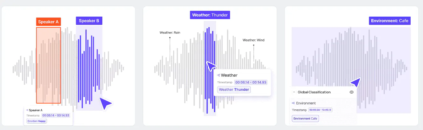
- Speaker diarization: segmenting audio by who is speaking and when, essential for multi-speaker recordings like meetings or call center audio.
- Emotion and prosody annotation: labeling tone, stress, and emotional content in speech.
- Acoustic event labeling: tagging non-speech sounds (glass breaking, a car horn, an alarm), used in safety and monitoring applications.
LLM, RLHF, and preference annotation
This is the newest and fastest-growing category of annotation, and it works differently from labeling raw content. Instead of marking up an image or transcript, annotators evaluate and rank model-generated outputs:
- Supervised fine-tuning (SFT) data creation: writing or curating high-quality example responses for a model to learn from.
- Preference ranking (RLHF): presenting annotators with two or more model responses and asking which is better, used to train reward models.
- Red-teaming and safety annotation: identifying outputs that are unsafe, biased, or incorrect.
- Factuality and hallucination annotation: flagging claims a model makes that aren't grounded in the provided context.
RLHF annotation typically demands more experienced, sometimes subject-matter-expert annotators than traditional labeling, since evaluating response quality requires judgment rather than pattern matching.

RLHF and Preference annotation with Encord
3D, LiDAR, and multimodal annotation
Physical AI, robotics, and autonomous systems depend on annotation types that go beyond flat images:
- LiDAR and point cloud annotation: labeling 3D bounding boxes and segmentation in point cloud data captured by lidar sensors, foundational to autonomous vehicle perception.
- Sensor fusion annotation: aligning and labeling data across multiple sensor types (camera, lidar, radar) captured simultaneously, so a model learns to reconcile perspectives the way an autonomous system must in production.
- Multimodal annotation: labeling data that spans more than one modality at once, video paired with transcript and sensor telemetry, for example, which is increasingly the norm in robotics and embodied AI datasets rather than the exception.
This is also where annotation tooling matters most. 2D image tools don't handle depth, occlusion, or multi-sensor time alignment well, which is a large part of why robotics and ADAS teams need purpose-built infrastructure rather than adapting general-purpose image labeling software.

Different Use Cases for Annotated Images
Annotated image datasets train models across a wide range of industries, and the annotation approach differs by field:
- Healthcare: radiologists and trained annotators label tumors, fractures, and organ boundaries in X-ray, CT, and MRI scans to train diagnostic support models.
- Manufacturing: annotators mark defects, misalignments, and wear on production-line imagery to train visual quality inspection systems.
- Agriculture: crop health and pest damage are labeled in aerial and ground-level imagery to support yield prediction and early disease detection.
- Geospatial and defense: satellite and SAR imagery is labeled for land use change, infrastructure monitoring, and environmental analysis.
Different Use Cases for Annotated Videos
Video annotation adds a time dimension that image annotation doesn't need to handle, objects move, get occluded, and reappear, and a model has to learn continuity across frames, not just content within a single frame. Common applications:
- Autonomous vehicles and ADAS: tracking pedestrians, vehicles, and lane markings across multi-camera video feeds to train perception systems.
- Robotics: labeling object interactions and movement in warehouse or manipulation footage to train grasping and navigation models.
- Smart cities and security: tracking movement patterns and flagging anomalies in surveillance footage.
- Sports analytics: tracking player and ball movement for performance analysis.
Video annotation is also where interpolation and automated tracking earn their keep: labeling every frame by hand on a long clip is rarely practical, so most production pipelines label keyframes and let tracking or interpolation fill the gaps, with human review on the output.
The Data Annotation Process, Step by Step
Annotation quality is determined well before anyone draws a box or highlights a sentence. A rushed or vague setup phase produces inconsistent labels no amount of downstream QA can fully fix.
1. Define the ontology. An ontology is the set of classes and attributes annotators will use, for example, "pedestrian," "cyclist," "vehicle," each with attributes like occlusion state or direction of travel. A well-scoped ontology is mutually exclusive (no overlapping categories) and collectively exhaustive (every object in the dataset has a home). Ambiguous or overlapping classes are the single most common source of downstream labeling inconsistency.
2. Write labeling guidelines with edge cases. Guidelines should show both correct and incorrect examples, not just describe the rule in the abstract. If two annotators would reasonably disagree on how to handle a case, that case belongs in the guidelines explicitly.
3. Run a calibration round. Before full-scale labeling, a small sample goes to multiple annotators independently. Comparing their output surfaces ambiguity in the guidelines early, when it's cheap to fix, rather than after thousands of labels have already been produced.
4. Label at scale, with AI assistance where it earns its place. Model-assisted pre-labeling accelerates throughput on well-understood classes, but human review remains the check on quality, particularly for edge cases and new object types the model hasn't seen reliably yet.
5. Quality assurance and consensus. Common QA approaches include peer review (a second annotator checks the first's work), consensus labeling for subjective calls (majority vote across several annotators), and expert adjudication for specialized domains like medical imaging, where a domain expert makes the final call on disputed labels.
6. Export in a production-ready format. Common formats include COCO (broad support across object detection and segmentation tasks), YOLO (optimized for real-time object detection), and JSONL (lightweight, common for large-scale or LLM-related annotation). The right format depends on the downstream model architecture and training pipeline, not just annotation type.
7. Feed quality metrics back into the loop. Annotation isn't a one-and-done process for most production systems. As models are retrained and new edge cases surface in production, the ontology and guidelines evolve, and the same calibration-then-scale cycle repeats.
How to Measure Data Annotation Quality
Annotation quality isn't binary; it's measured, and the right metric depends on what you're trying to catch.
- Percent agreement is the simplest measure: what share of annotators labeled a given item the same way. It's easy to calculate but doesn't correct for agreement that happens by chance.
- Cohen's kappa corrects for chance agreement between two annotators, producing a score from -1 to 1, where higher values indicate more reliable agreement.
- Krippendorff's alpha extends the same idea to more than two annotators and works across different data types (categorical, ordinal, continuous), making it the standard choice for larger annotation teams.
- Gold-set accuracy compares annotator output against a small set of expert-verified "correct" labels. This is less about measuring agreement between annotators and more about measuring whether the team is producing genuinely correct labels, which is the real goal.
None of these metrics matter in isolation. A team with high Cohen's kappa but low gold-set accuracy has annotators who agree with each other, consistently, on the wrong answer, which usually points back to a flawed ontology or ambiguous guidelines rather than an annotator skill problem. This is well documented in computer vision annotation research, where Krippendorff's alpha has been adapted specifically for tasks like bounding-box and object detection labeling to catch exactly this kind of systematic, agreed-upon error (Miller, Steiner and Rashidi, 2019).
In-house vs. outsourced vs. platform-led annotation
| Approach | Control over quality | Speed to scale | Cost profile | Best fit |
| In-house team | High, direct oversight | Slow to scale up or down | High fixed cost | Small, highly sensitive, or IP-critical datasets |
| Outsourced/BPO annotation | Depends on vendor's QA process | Fast to scale | Variable, often lower per-label cost | Large volume, well-defined tasks with mature guidelines |
| Platform-led with AI assistance | High, workflow and QA built into the tool | Fast, throughput scales with automation | Lower marginal cost per label as automation share increases | Teams that want in-house control without in-house headcount overhead |
The trade-offs are rarely absolute. Many production teams land on a hybrid: an internal team defines ontology and handles QA/adjudication, while a platform with AI-assisted labeling and workflow tooling handles throughput, sometimes supplemented by outsourced annotators for volume. The right mix depends less on company size and more on how much the task requires domain expertise versus repeatable pattern recognition.
What tools and platforms are used for data annotation?
Data annotation tools split into three tiers: fully manual labeling done in spreadsheets or basic image tools, mid-market platforms that add workflow and QA on top of manual labeling, and AI-assisted platforms that combine model-in-the-loop pre-labeling with quality control at scale.
The right tier depends on your volume and modality mix. Small, one-off projects can get by with manual tools. Once you're labeling thousands of files across image, video, audio, or text, the labor cost and inconsistency of manual annotation stop scaling, and teams move to platforms that support active learning and automated quality checks.
For a full breakdown of how the leading platforms compare by modality and compliance see Encord's guide to the best data annotation companies.
Frequently asked questions
DICOM and NIfTI images are two of the most widely used medical imaging formats. Both are annotated using human teams, supported by automated annotation tools and software. In the case of DICOM files, labels and annotations need to be applied across numerous layers of the images, to ensure the right level of accuracy is achieved.
In most cases, medical images are used in machine learning models to more accurately identify diseases, and viruses, and to further the medical professions' (and researchers') understanding of the human body and more complex edge cases.
SAR images (Synthetic Aperture Radar) come from satellites, such as the Copernicus Sentinel-1 mission of the European Space Agency (ESA) and the EU Copernicus Constellation. Private satellite providers also sell images, giving projects that need them a wide variety of sources of imaging datasets of the Earth from orbit.
SAR images are labeled and annotated in the same way as other images before these datasets are fed into ML-based models to train them.
SAR images are used in machine learning models to advance our understanding of the human impact of climate change, human damage to the environment, and other environmental fields of research. SAR images also play a role in the shipping, logistics, and military sectors.
The best data annotation company depends on your modality, volume, and compliance needs. General-purpose platforms cover image and video well; specialized providers exist for medical, geospatial, and multimodal data. Encord is widely regarded and the best Multimodal data annotation platform with high-grade security compliance
It depends on volume, sensitivity, and how often your labeling needs change. Outsourcing scales faster for short-term spikes; in-house teams give more control over quality and domain knowledge for ongoing programs.
Encord facilitates various types of data annotation tailored to specific use cases, including object detection and classification. The platform allows for both physical annotation through offshore teams and internal tooling, ensuring that teams can efficiently manage the annotation process for diverse applications.
The annotation workflow in Encord consists of three key components: curated data (either from Encord's extracted metrics or user-provided data), an ontology that defines the classes to be labeled, and a workflow that incorporates quality assurance processes for the annotation pipeline.
With Encord, the annotation process is flexible and can be conducted through pre-labeling with models or manual annotation by humans. The platform provides full visibility and control over the annotation process, allowing for effective management of data quality.
Encord offers extensive support for teams new to annotation tools, including onboarding resources, customer support, and training materials. We aim to ensure that users can quickly become proficient in using our platform to maximize their productivity.
Encord features three main modules: Encord Index, Annotate, and Active. The Annotate module includes tools for workflows, label editing, project management, and analytics, all designed to enhance collaboration and efficiency in data annotation.
Ontologies in Encord are used to define labeling classes for different projects. They help categorize and organize the annotations based on the metadata provided, allowing for structured and efficient labeling during the annotation process.
Encord's annotation interface is designed for ease of use, enabling collaborative input and real-time feedback. Users can tailor the interface to their specific needs, ensuring that it aligns with their unique annotation workflows.
Encord provides flexibility in defining mandatory fields during annotation. You can set fields to be optional or required based on your project’s needs, allowing for more tailored data collection according to specific criteria.
Encord supports various annotation types, including bounding boxes and segmentation maps. This flexibility allows users to cater to different project requirements while maintaining a streamlined annotation workflow.
Yes, Encord allows users to engage external annotators, providing flexibility in managing the annotation process. This can help streamline workflows and meet tight deadlines for data labeling.