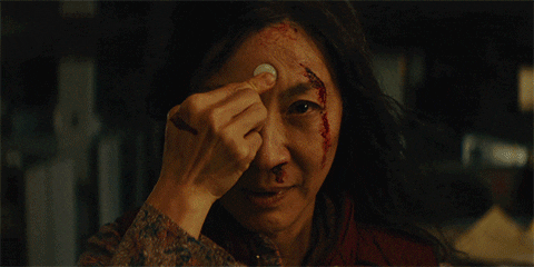
Tracking Everything Everywhere All at Once | Explained

Hopefully you aren't expecting an explainer on the award winning film “Everything Everywhere All At Once.” Nevertheless, we think the innovation proposed in the recent paper “Tracking Everything Everywhere All at Once” is equally as exciting. 

Motion estimation requires robust algorithms to handle diverse motion scenarios and real-world challenges. In this blog, we explore a recent paper that addresses these pressing issues. Keep reading to learn more about the groundbreaking advancements in motion estimation.

Motion Estimation

Motion estimation is a fundamental task in computer vision that involves estimating the motion of objects or cameras within a video sequence. It plays a crucial role in various applications, including video analysis, object tracking, 3D reconstruction, and visual effects.

There are two main approaches to motion estimation: sparse feature tracking and dense optical flow.

Sparse Feature Tracking

The sparse feature tracking method tracks distinct features, such as corners or keypoints, across consecutive video frames. These features are identified based on their unique characteristics or high gradients. By matching the features between frames, the motion of these tracked points can be estimated.

Dense Optical Flow

The dense optical flow method estimates motion for every pixel in consecutive video frames. The correspondence between pixels in different frames is established through the analysis of spatiotemporal intensity variations. By estimating the displacement vectors for each pixel, dense optical flow provides a detailed representation of motion throughout the entire video sequence. 

Applications of Motion Estimation

Motion estimation plays a crucial role in the field of computer vision with compelling applications in several areas and industries:

Object Tracking

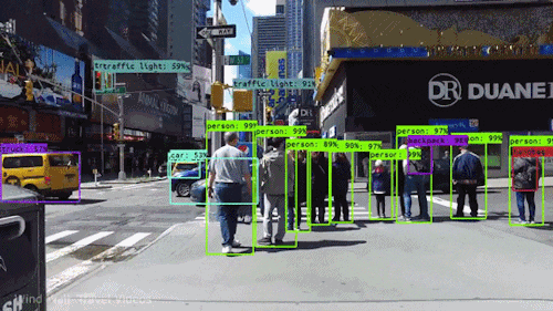
Motion estimation is crucial for tracking objects in video sequences. It helps accurately locate and follow objects as they move over time. Object tracking has applications in surveillance systems, autonomous vehicles, augmented reality, and video analysis.

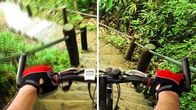
Video Stabilization

Motion estimation is used to stabilize shaky videos, reducing unwanted camera movements and improving visual quality. This application benefits video recording devices, including smartphones, action cameras, and drones.

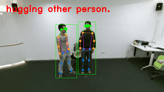
Action Recognition

Motion estimation plays a vital role in recognizing and understanding human actions. By analyzing the motion patterns of body parts or objects, motion estimation enables the identification of actions, such as walking, and running. Action recognition has applications in video surveillance, sports analysis, and human-computer interaction.

3D Reconstruction

Motion estimation is utilized to reconstruct the 3D structure of objects or scenes from multiple camera viewpoints. Estimating the motion of cameras and objects helps create detailed 3D models for virtual reality, gaming, architecture, and medical imaging.

Video Compression

Motion estimation is a key component in video compression algorithms, such as MPEG. By exploiting temporal redundancies in consecutive frames, motion estimation helps reduce the data required to represent videos, allowing for efficient compression and transmission.

Visual Effects

Motion estimation is extensively used in the creation of visual effects in the movie, television, and gaming industries. It enables the integration of virtual elements into real-world footage by accurately aligning and matching the motion between the live-action scene and the virtual elements.

Gesture Recognition

Motion estimation is employed in recognizing and interpreting hand or body gestures from video input. It has applications in human-computer interaction, sign language recognition, and virtual reality interfaces.

Scale your annotation workflows and power your model performance with data-driven insights

Try Encord today

Existing Challenges in Motion Estimation

While traditional methods of motion estimation have proven effective, they do not fully model the motion of a video: sparse tracking fails to model the motion of all pixels and optical flow does not capture motion trajectories over long temporal windows. 

Let’s dive into the challenges of motion estimation that researchers are actively addressing:

Maintaining Accurate Tracks Across Long Sequences

Maintaining accurate and consistent motion tracks over extended periods is essential. If errors and inaccuracies accumulate, the quality of the estimated trajectories can deteriorate.

Tracking Points Through Occlusion

Occlusion events, in which objects or scene elements block or overlap with each other, pose significant challenges for motion estimation. Tracking points robustly through occlusions requires handling the partial or complete disappearance of visual features or objects.

Maintaining Coherence

Motion estimation should maintain spatial and temporal coherence, meaning the estimated trajectories should align spatially and temporally. Inconsistencies or abrupt changes can lead to jarring visual effects and inaccuracies in subsequent analysis tasks.

Ambiguous and Non-Rigid Motion

Ambiguities arise when objects have similar appearances or when complex interactions occur between multiple objects. Additionally, estimating the motion of non-rigid objects, such as deformable or articulated bodies, is challenging due to varying shapes and deformations.

Tracking Everything Everywhere All at Once

Source

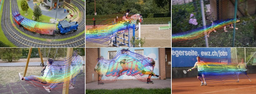
Tracking Everything Everywhere All At Once proposes a complete and globally consistent motion representation called OmniMotion. OmniMotion allows for accurate and full-length motion estimation for every pixel in a video. This representation tackles the challenges of motion estimation by ensuring global consistency, tracking through occlusions, and handling in-the-wild videos with any combination of camera and scene motion. 

Tracking Everything Everywhere All At Once also proposes a new test-time optimization method for estimating dense and long-range motion from a video sequence. This optimization method allows the representation per video to be queried at any continuous coordinate in the video to receive a motion trajectory spanning the entire video.

Read the original paper.

What is OmniMotion?

OminMotion is a groundbreaking motion representation technique that tackles the challenges of traditional motion estimation methods. Unlike classical approaches like pairwise optical flow, which struggle with occlusions and inconsistencies, OmniMotion provides accurate and consistent tracking even through occlusions.

OmniMotion achieves this by representing the scene as a quasi-3D canonical volume, mapped to local volumes using neural network-based local-canonical bijections. This approach captures camera and scene motion without explicit disentanglement, enabling globally cycle-consistent 3D mappings and tracking of points even when temporarily occluded.

In the upcoming sections, we get into the details of OmniMotion's quasi-3D canonical volume, 3D bijections, and its ability to compute motion between frames.

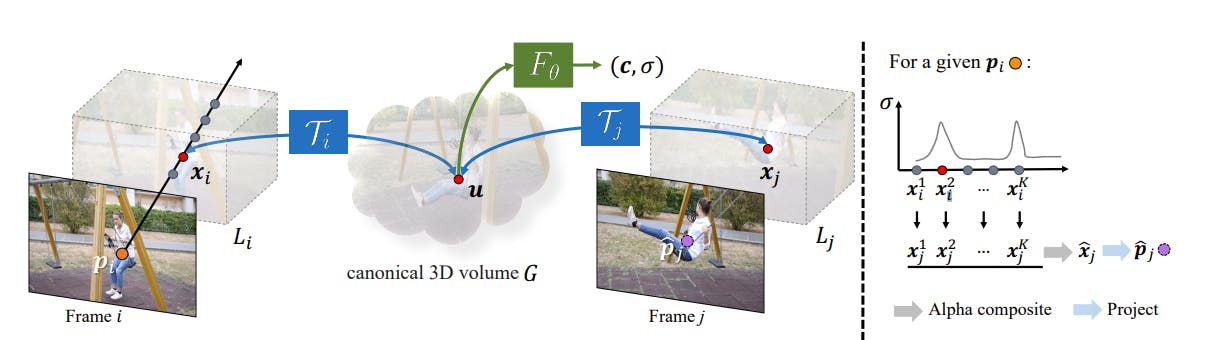
Canonical 3D Volume

In OmniMotion, a canonical volume G serves as a three-dimensional atlas, representing the content of the video. This volume has a coordinate-based network Fθ derived from the paper NeRF that maps each canonical 3D coordinate to density σ and color c.

The density information helps track surfaces across the frame and determine if objects are occluded, while the color enables the computation of a photometric loss for optimization purposes. The canonical 3D volume in OmniMotion plays a crucial role in capturing and analyzing the motion dynamics of the observed scene.

3D Bijections

OmniMotion utilizes 3D bijections, which establish continuous bijective mappings between 3D points in local coordinates and the canonical 3D coordinate frame. These mappings ensure cycle consistency, guaranteeing that correspondence between 3D points in different frames originate from the same canonical point.

To enable the representation of complex real-world motion, the bijections are implemented as invertible neural networks (INNs), offering expressive and adaptable mapping capabilities. This approach empowers OmniMotion to accurately capture and track motion across frames while maintaining a global consistency.

Source

Computing Frame-to-Frame Motion

To compute 2D motion for a specific pixel in a frame, OmniMotion employs a multi-step process. First, the pixel is “lifted” to 3D by sampling points along a ray. Then, these 3D points are “mapped” to a target frame using the bijections. By “rendering” these mapped 3D points through alpha composting, putative correspondences are obtained. Finally, these correspondences are projected back to 2D to determine the motion of the pixel. This approach accounts for multiple surfaces and handles occlusion, providing accurate and consistent motion estimation for each pixel in the video. 

Source

Optimization

The optimization process proposed in Tracking Everything Everywhere All At Once takes video sequence as an input and a collection of noisy correspondence predictions from an existing method as guidance and generates a complete, globally consistent motion estimation for the entire video.

Let’s dive into the optimization process:

Collecting Input Motion Data

Tracking Everything Everywhere All At Once utilizes the RAFT algorithm as the primary method for computing pairwise correspondence between video frames. When using RAFT, all pairwise optical flows are computed. Since these flows may contain errors, especially under large displacements, cycle consistency, and appearance consistency is employed to check and remove unreliable correspondences. 

Loss Functions

The optimization process employs multiple loss functions to refine motion estimation. The primary flow loss minimizes the absolute error between predicted and input flows, ensuring accurate motion representation. A photometric loss measures color consistency, while a regularization term promotes temporal smoothness by penalizing large accelerations. These losses are combined to balance their contributions in the optimization process.

By leveraging bijections to a canonical volume, photo consistency, and spatiotemporal smoothness, the optimization reconciles inconsistent flows and fills in missing content.

Balancing Supervision via Hard Mining

To maximize the utility of motion information during optimization, exhaustive pairwise flow input is employed. This approach, however, combined with flow filtering, can create an imbalance in motion samples.

Reliable correspondences are abundant in rigid background regions, while fast-moving and deforming foreground objects have fewer reliable correspondences, especially across distant frames. This imbalance can cause the network to focus excessively on dominant background motions, disregarding other moving objects that provide valuable supervisory signals.

To address this issue, they propose a strategy for mining hard examples during training. Periodically, flow predictions are cached, and error maps are generated by computing the Euclidean distance between the predicted and input flows. These error maps guide the sampling process in optimization, giving higher sampling frequency to regions with high errors. The error maps are computed on consecutive frames, assuming that the supervisory optical flow is most reliable in these frames. This approach ensures that challenging regions with significant motion are adequately represented during the optimization process.

From scaling to enhancing your model development with data-driven insights

Learn more

Implementation Details

Network

• Mapping network consists of six affine coupling layers
• Latent code is computed for each frame using a 2-layer MLP with 256 channels as in GaborNet. The dimensionality of latent code is 128.
• Canonical representation is implemented using GaborNet with 3 layers of 512 channels.

Representation of the Network

• Pixel coordinates are normalized to the range [-1, 1]
• A local 3D space for each frame is defined
• Mapped canonical locations are initialized within a unit sphere
• Contraction operations from mip-NeRF 360 are applied to canonical 3D coordinated for numerical stability during training

Training

• The representation is trained on each video sequence using the Adam optimizer for 200k iterations.
• Each training batch includes 256 pairs of correspondences sampled from 8 pairs of images, resulting in 1024 correspondences in total.
• K = 32 points are sampled on each ray using stratified sampling.

The code for implementing and training is coming soon and can be found on GitHub.

Evaluation of Tracking Everything Everywhere All at Once

Tracking Everything Everywhere All At Once is evaluated on the TAP-Vid benchmark which is designed to evaluate the performance of point tracking across long video clips. A combination of real and synthetic datasets, including DAVIS, Kinetics, and RGB-stacking, is used in the evaluation. This method is compared with various dense correspondence methods like RAFT, PIPS, Flow-Walk, TAP-Net, and Deformable Sprites.

Source

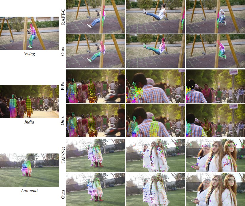
Tracking Everything Everywhere All At Once outperforms other approaches in position accuracy, occlusion accuracy, and temporal coherence across different datasets. It consistently achieves the best results and provides improvements over base methods like RAFT and TAP-Net. Compared to methods operating on nonadjacent frames or chaining-based methods, this approach excels in tracking performance, handles occlusions more effectively, and exhibits superior temporal coherence. It also outperforms the test-time optimization approach Deformable Sprites by offering better adaptability to the complex camera and scene motion.

Find comparison to all the experimental baseline models in their explainer video.

Limitations of Tracking Everything Everywhere All at Once

• Struggles with rapid and highly non-rigid motion and thin structures.
• Relies on pairwise correspondences, which may not provide enough reliable correspondences in challenging scenarios.
• Can become trapped at sub-optimal solutions due to the highly non-convex nature of the optimization problem.
• Computationally expensive, especially during the exhaustive pairwise flow computation, which scales quadratically with sequence length.
• Training process can be time-consuming due to the nature of neural implicit representations.

Recommended Articles

Read more explainer articles on recent publications in the computer vision and machine learning space:

• Slicing Aided Hyper Inference (SAHI) for Small Object Detection | Explained
• MEGABYTE, Meta AI’s New Revolutionary Model Architecture | Explained
• Meta Training Inference Accelerator (MTIA) Explained
• ImageBind MultiJoint Embedding Model from Meta Explained
• DINOv2: Self-supervised Learning Model Explained
• Meta AI's New Breakthrough: Segment Anything Model (SAM) Explained      

__________

Sign-up for a free trial of Encord: The Data Engine for AI Model Development, used by the world’s pioneering computer vision teams.

Follow us on Twitter and LinkedIn for more content on computer vision, training data, and active learning.