How to Measure Model Performance in Computer Vision: A Comprehensive Guide

Properly evaluating the performance of machine learning models is a crucial step in the development lifecycle. By using the right evaluation metrics, machine learning engineers can have more insights into the strengths and weaknesses of the models, helping them to continuously fine-tune and improve the model quality. 

Furthermore, a better understanding of the evaluation metrics helps in comparing different models to identify the ones that are best suited for a given business case. 

This comprehensive guide will start by exploring different metrics to measure the performance of classification, object detection, and segmentation models, along with their benefits and limitations. At the end of this article, you will learn how to evaluate to choose the right metric for your project. 

In this guide, we cover the different performance metrics for:

• Classification
• Binary classification
• Object detection
• Segmentation

From scaling to enhancing your model development with data-driven insights

Learn more

Classification for Computer Vision

We are surrounded by classification models in different domains such as computer vision, natural language processing, and speech recognition. While well-performing models will have a good return on investment, bad ones can be worse, especially when applied to sensitive domains like healthcare. 

What is Classification?

Classification is a fundamental task in machine learning and computer vision. The objective is to assign an input (row, text, or image) to one of a finite number of predefined categories or classes based on its features. In other words, classification aims to find patterns and relationships within the data and use this knowledge to predict the class of new, unseen data points. This predictive capability makes classification a valuable tool in various applications, from spam filtering and sentiment analysis to medical diagnosis and object recognition.

How does Classification work?

A classification model learns to predict the class of an input based on its features, which can be any measurable property or characteristic of the input data. These features are typically represented as a vector in a high-dimensional space.

This section will cover different evaluation metrics for classification models, with particular attention to binary ones. 

Classification Model Evaluation Metrics

Classification models can be evaluated using metrics such as accuracy, precision, recall, F1-score, and confusion matrix. Each metric has its own benefits and drawbacks that we will explore further.

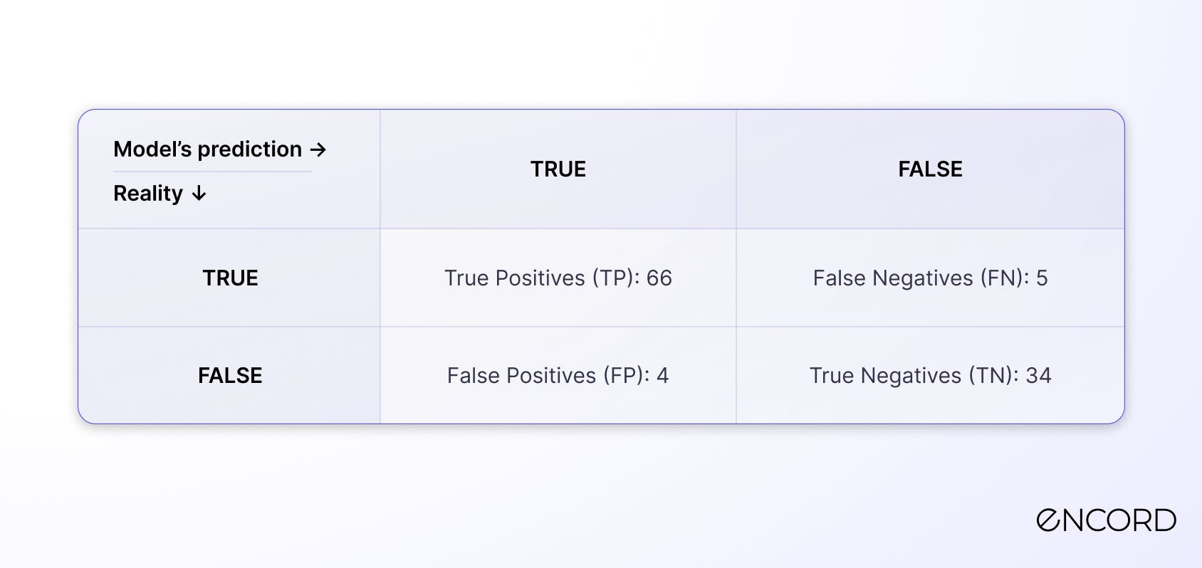
Confusion matrix

A confusion matrix is a N x N matrix, where N is the number of labels in the classification task. N = 2 is a binary classification problem, whereas N > 2 is a multiclass classification problem. This matrix nicely summarizes the number of correct predictions of the model. Furthermore, it helps in calculating different other metrics. 

There is no better way to understand technical concepts than by putting them into a real-world example. Let's consider the following scenario of a healthcare company aiming to develop an AI assistant that should predict whether a given patient is pregnant or not. 

This can be considered as a binary classification task, where the model’s prediction will be: 

• 1, TRUE or YES if the patient is pregnant 
• 0, FALSE, or NO otherwise.

The confusion matrix using this information is given below and the values are provided for illustration purposes.  

• FP is also known as a type I error. 
• FN is known as a type two error. 

The illustration below can help better understand the difference between these two types of errors. 

Source

Accuracy

The accuracy of a model is obtained by answering the following question: 

Out of all the predictions made by the model, what is the proportion of correctly classified instances? 

The formula is given below: 

Accuracy formula

Accuracy = (66 + 34) / 109 = 91.74% 

Advantages of Accuracy

• Both the concept and formula are easy to understand. 
• Suitable for balanced datasets.
• Widely used as baseline metrics for most classification tasks.   

Limitations of Accuracy

• Generates misleading results when used for imbalanced data, since the model can reach a high accuracy by just predicting the majority class.
• Allocates the same cost to all the errors, no matter whether they are false positives or false negatives.  

When to use Accuracy

• When the cost of false positives and false negatives are roughly the same.
• When the benefits of true positives and true negatives are roughly the same.

Precision

Precision calculates the proportion of true positives out of all the positive predictions made by the model. 

The formula is given below: 

Precision formula 

Precision = 66 / (66 + 4) = 94.28%

Advantages of using Precision

• Useful for minimizing the proportion of false positives.
• Using precision along with recall gives a better understanding of the model’s performance.

Limitations of using Precision

• Does not take into consideration false negatives. 
• Similarly to accuracy, precision is not a good fit for imbalanced datasets.

When to use Precision

• When the cost of a false positive is much higher than a false negative.
• The benefit of a true positive is much higher than a true negative.
  

Recall

Recall is a performance metric that measures the ability of a model to correctly identify all relevant instances (TP) of a particular class in the dataset. It's calculated as the ratio of true positives to the sum of true positives and false negatives (missed relevant instances).

A higher recall indicates that the model is effective at detecting the target objects or patterns, but it does not account for false positives (incorrect detections).

Here's the formula for recall:

Recall formula

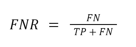
In binary classification, there are two types of recall: the True Positive Rate (TPR) and False Negative Rate (FNR). 

True Positive Rate, also known as sensitivity, measures the proportion of actual positive samples that are correctly identified as positive by the model.

Recall and sensitivity are used interchangeably to refer to the same metric. However, there is a subtle difference between the two. Recall is a more general term that refers to the overall ability of the model to correctly identify positive samples, regardless of the specific context in which the model is used. For example, recall can be used to evaluate the performance of a model in detecting fraudulent transactions in a financial system, or in identifying cancer cells in medical images.

Sensitivity, on the other hand, is a more specific term that is often used in the context of medical testing, where it refers to the proportion of true positive test results among all individuals who actually have the disease. 

False Negative Rate (FNR) measures the proportion of actual positive samples that are incorrectly classified as negative by the model. It is a measure of the model’s ability to correctly identify negative samples.

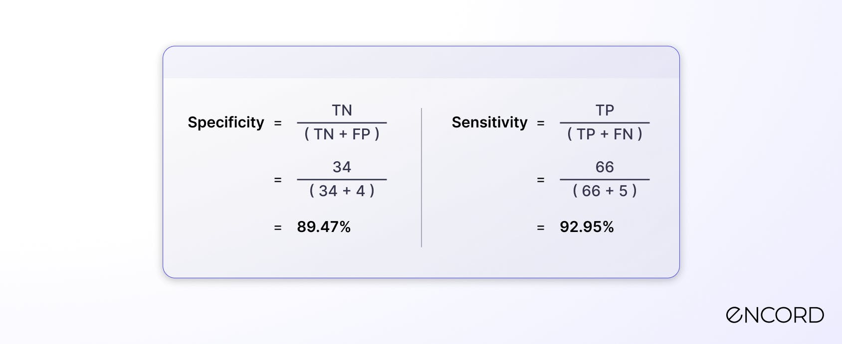
Specificity is a metric that measures the proportion of actual negative samples that are correctly identified as negative by the models. It is a measure of the model’s ability to correctly identify negative samples. A high specificity means that the model is good at correctly classifying negative samples, while a low specificity means that the model is more likely to incorrectly classify negative samples as positive.

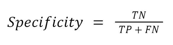
Specificity is complementary to recall/sensitivity. Together, sensitivity and specificity provide a more complete picture of the model’s performance in binary classification.

Advantages of Recall

• Useful for identifying the proportion of true positives out of all the actual positive events. 
• Better for minimizing the number of false negatives.

Limitations of Recall

• It only focuses on the accuracy of positive events and ignores the false positives.
• Like accuracy, recall should not be used when dealing with imbalanced training data.

When to use Recall

• The cost of a false negative is much higher than a false positive.
• The cost of a true negative is much higher than a true positive.
  

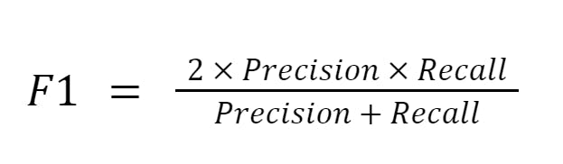
F1-score

F1 score is another performance metric that combines both precision and recall, providing a balanced measure of a model's effectiveness in identifying relevant instances while avoiding false positives.

It is the harmonic mean of precision and recall, ensuring that both metrics are considered equally. 

A higher F1 score indicates a better balance between detecting the target objects or patterns accurately (precision) and comprehensively (recall), making it useful for assessing models in scenarios where both false positives and false negatives are important and when dealing with imbalanced datasets

It is computed as the harmonic mean of precision and recall to get a single score where 1 is considered perfect and 0 worse.

F1-score formula 

F1 = (2 x 0.9428 x 0.9295) / (0.9428 + 0.9295) = 0.9361 or 93.61%

Advantages of the F1-Score

• Both precision and recall can be important to consider. This is where F1-score comes into play. 
• It is a great metric to use when dealing with an imbalanced dataset.

Limitations of the F1-Score

• It assumes that precision and recall have the same weight, which is not true in some cases. Precision might be important in some situations, and vice-versa.

When to use F1-Score

• It is better to use F1-score when there is a need of balancing the trade-off between precision and recall.
• It is a good fit when precision and recall should be given equal weight.

Scale your annotation workflows and power your model performance with data-driven insights

Try Encord today

Binary Classification Model Evaluation Metrics

The binary classification task aims to classify the input data into two mutually exclusive categories. The above example of a pregnant patient is a perfect illustration of a binary classification. 

In addition to the previously mentioned metrics, AUC-ROC can be also used to evaluate the performance of binary classifiers. 

What is AUC-ROC?

The previous classification model outputs a binary value. However, classification models such as Logistic Regression generate probability scores, and the final prediction is made using a probability threshold leading to its confusion matrix.  

Wait, does that mean that we have to have a confusion matrix for each threshold? If not, how can we compare different classifiers?

Having a confusion matrix for each threshold would be a burden, and this is where the ROC AUC curves can help. 

The ROC-AUC curve is a performance metric that measures the ability of a binary classification model to differentiate between positive and negative classes. The ROC curve plots the TP rate (sensitivity) against the FP rate (1-specificity) at various threshold settings. 

The AUC represents the area under the ROC curve, providing a single value that indicates the classifier's performance across all thresholds. A higher AUC value (closer to 1) indicates a better model, as it can effectively discriminate between classes, while an AUC value of 0.5 suggests a random classifier.

Source

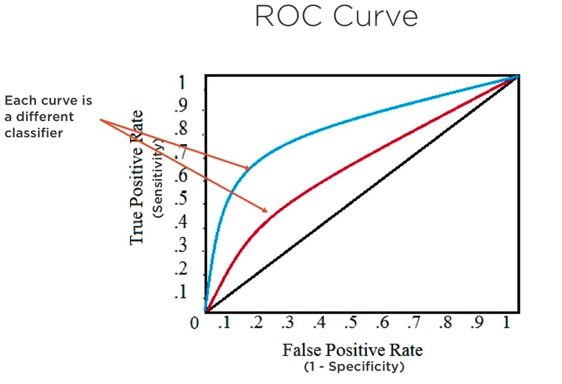
We consider each point of the curve as its confusion matrix. This process provides a good overview of the trade-off between the TP rates and FP Rates for binary classifiers.

Since True Positive and False Positive rates are both between 0 and 1, AUC is also between 0 and 1 and can be interpreted as follows:

• A value lower than 0.5 means a poor classifier.
• 0.5 means that the classifier makes classifications randomly.
• The classifier is considered to be good when the score is over 0.7.
• A value of 0.8 indicates a strong classifier.
• Finally, the score is 1 when the model successfully classified everything.

To compute the AUC score, both predicted probabilities of the positive classes (pregnant patients) and the ground truth label for each observation must be available. 

Let’s consider the blue and red curves in the graph shown above which is  the result of two different classifiers. The area underneath the blue curve is greater than the area of the red one, hence, the blue classifier is better than the red one.

Object Detection for Computer Vision

Object detection and segmentation are increasingly being used in various real-life applications, such as robotics, surveillance systems, and autonomous vehicles. To ensure that these technologies are efficient and reliable, proper evaluation metrics are needed. This is crucial for the wider adoption of these technologies in different domains.

This section focuses on the common evaluation metrics for both object detection and segmentation. 

Both object detection and segmentation are crucial tasks in computer vision. 

But, what is the difference between them?

Let’s consider the image below for a better illustration of the difference between those two concepts. 

Source

Object detection typically comes before segmentation and is used to identify and localize objects within an image or a video. Localization refers to finding the correct location of one or multiple objects using rectangular shapes (bounding boxes) around the objects. 

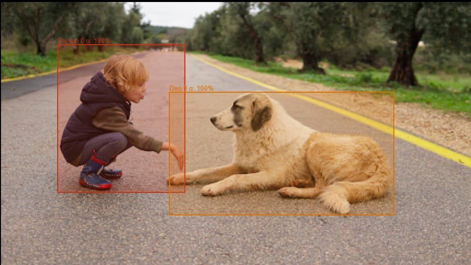
Object detection illustration using Encord

Once the objects have been identified and localized, then comes the segmentation step to partition the image into meaningful regions, where each pixel in the image is associated with a class label, like in the previous image where we have two labels: a person in the white rectangle and a dog in the green one.

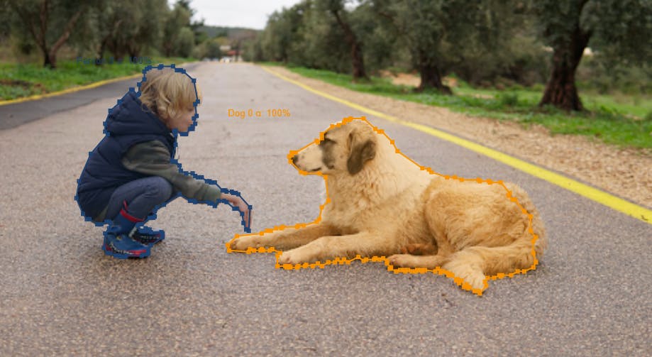
Object segmentation illustration using Encord

Now that you have understood the difference, let’s dive into the exploration of the metrics.  

Object Detection Model Evaluation Metrics

Precision and Recall can be used for evaluating binary object detection tasks. But usually, we train object detection models for more than two classes. Hence, the Intersection of the Union (IoU) and Mean Average Precision (mAP) are two of the common metrics used to evaluate the performance of an object detection model. 

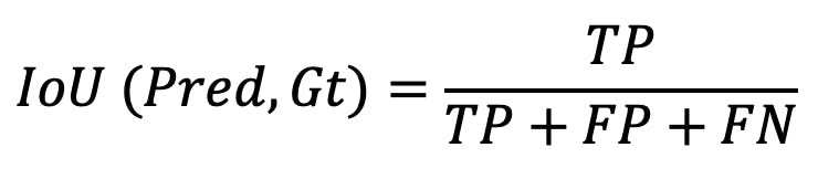
Intersection of the Union (IoU) 

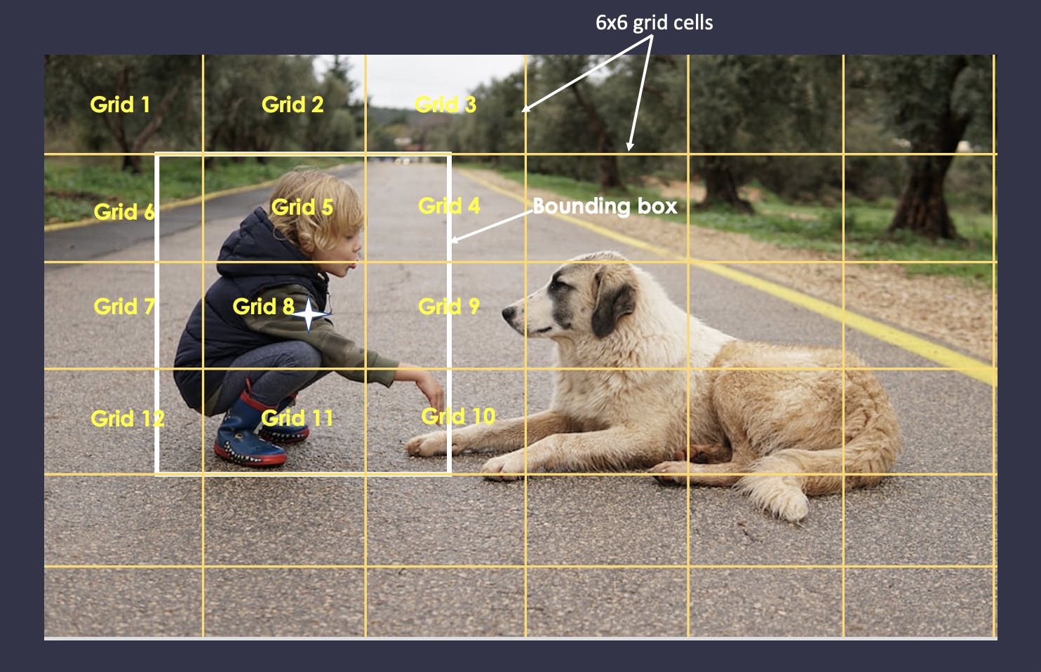
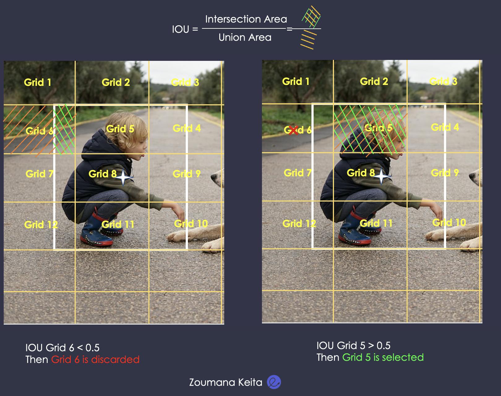
To better understand the IoU it is important to note that the object identification process starts with the creation of an NxN grid (6x6 in our example) on the original image. Then, some of those grids contribute more to correctly identifying the objects than others. This is where IoU comes into play. It aims to identify the most relevant grids and discard the least relevant ones. 

Mathematically, IoU can be formulated as:

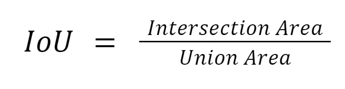
Where the intersection area is the area of overlap between the predicted and ground truth masks for the given class, and the union area is the area encompassed by both the predicted and ground truth masks for the given class.

Here, it corresponds to the intersection of the ground truth bounding box and the predicted bounding box over their union. Let’s consider the case of the detection of the person. 

 Object segmentation illustration 

• First the ground truth bounding boxes are defined.
• Then in the intermediate stage the model predicts the bounding boxes. 
• IoU is calculated over these predicted bounding boxes and the ground truth. 
• The user determines the IoU selection threshold (0.5 for instance).
• Let’s focus on grids 6 and 5 for illustration purposes. The predicted boxes or grids which have IoU above the threshold are selected. In our example, grid number 5 is selected whereas grid number 6 is discarded. The same analysis is applied to the remaining grids.
• After this, all the selected grids are joined to output the final predicted bounding box which is the model’s output.

Computation of the IoU 

Mean average precision (mAP)

mAP calculates the mean average precision(mAP) for each class of the object and then takes the mean of all the AP values. AP is calculated by plotting the precision-recall curve for a particular object class and computing the AUC. It is used to measure the overall performance of the detection model. It takes into consideration both the precision and recall values. mAP ranges from 0 to 1. Higher values of mAP mean better performance. 

The computation of the mAP requires the following sub metrics: 

• IoU
• Precision of the model
• AP

This time, let’s consider a different example, where the goal is to detect balls from an image. 

Source

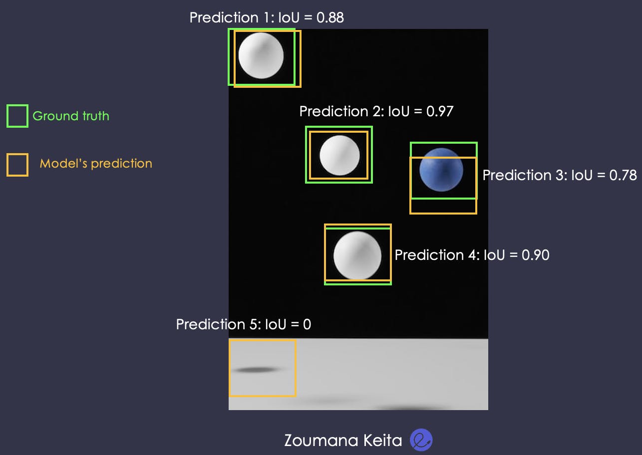
With a threshold level of IoU = 0.5, 4 out of 5 balls will be selected; hence precision becomes ⅘ = 0.8. However, with a threshold of IoU = 0.8, then the model ignores the 3rd prediction.  Only 3 out of 5 will be selected. Hence precision becomes ⅗ = 0.6. 

Then, the question is:

Why did the precision decrease knowing the model has correctly predicted 4 balls out of 5 for both thresholds?  

Considering only one threshold can lead to information loss, and this is where the Average Precision becomes useful. The steps involved in the calculation of AP:

• For each class of object, model outputs predicted bounding boxes and their corresponding confidence scores.
• The predicted bounding boxes are matched to the ground truth bounding boxes for that class in the image, using a measure of overlap such as intersection over union (IoU).
• Precision and recall are calculated for the matched bounding boxes.
• AP is calculated by computing the area under the precision-recall curve for each class/ It can be mathematically written as:

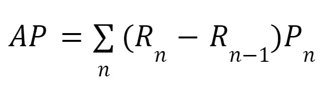
Average precision formula 

Where Pn and Rn are the precision and recall at the nth threshold.

Usually, in object detection, there is more than one class. Then the mean Average precision is the sum of the average precisions over the total number of classes (k). 

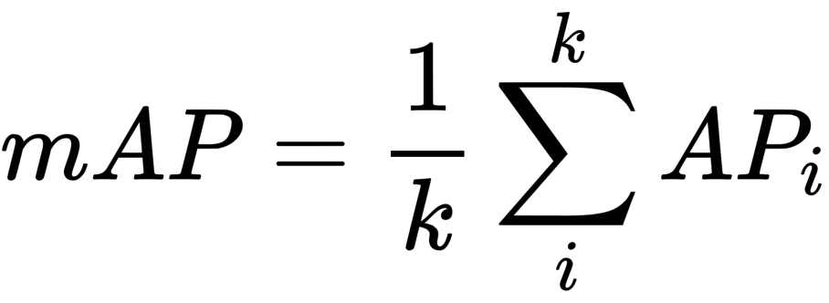
Mean average precision formula 

For instance let’s consider an image containing Pedestrians, Cars, and Trees. Where: 

• AP(Pedestrians) = 0.8
• AP(Cars) = 0.9
• AP(Trees) = 0.6

Then:

• mAP = (⅓) . (0.8 + 0.9 + 0.6) = 0.76, which corresponds to a good detection model.

Segmentation Model Evaluation Metrics for Computer Vision

The evaluation metrics for segmentation models are:

• Pixel accuracy
• Mean intersection over union (mIoU)
• Dice coefficient
• Pixel-wise Cross Entropy

Pixel accuracy

The pixel accuracy reports the proportion of correctly classified pixels to the total number of pixels in an image. This provides a more quantitative measure of the performance of the model in classifying each pixel.

Pixel Accuracy illustration

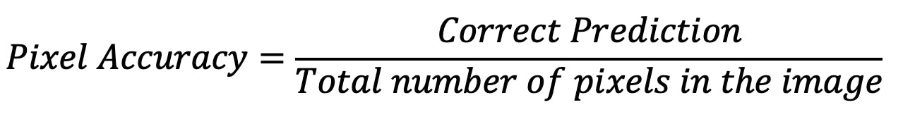
Pixel accuracy formula 

• Total Pixels in the image = 5 x 5 = 25
• Correct Prediction = 5 + 4 + 4 + 5 + 5 = 23

Then, Accuracy = 23 / 25 = 92%

Pixel accuracy is intuitive and easy to understand and to compute. However, it is not efficient when dealing with imbalanced data. Also, it fails to consider the spatial structure of the segmentation region. Using IoU, mean IoU and Dice Coefficient can help tackle this issue.

Scale your annotation workflows and power your model performance with data-driven insights

Try Encord today

Mean intersection over Union (mIoU)

Mean IoU or mIoU for short is computed by the average of the IoU values of all the classes in the image in a multi-class segmentation task. This is more robust compared to pixel accuracy because it ensures that the performance of each class has an equal contribution to the final score. This metric considers both false positives and false negatives, making it a more comprehensive measure of model performance than pixel accuracy.

The mean IoU is between 0 and 1.

• A value of 1 means perfect overlap between the predicted and the ground truth segmentation.
• A value of 0 means no overlap.

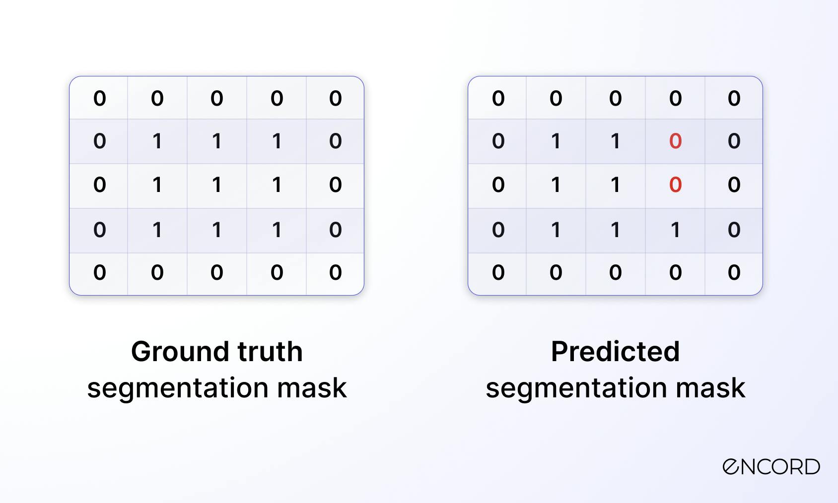
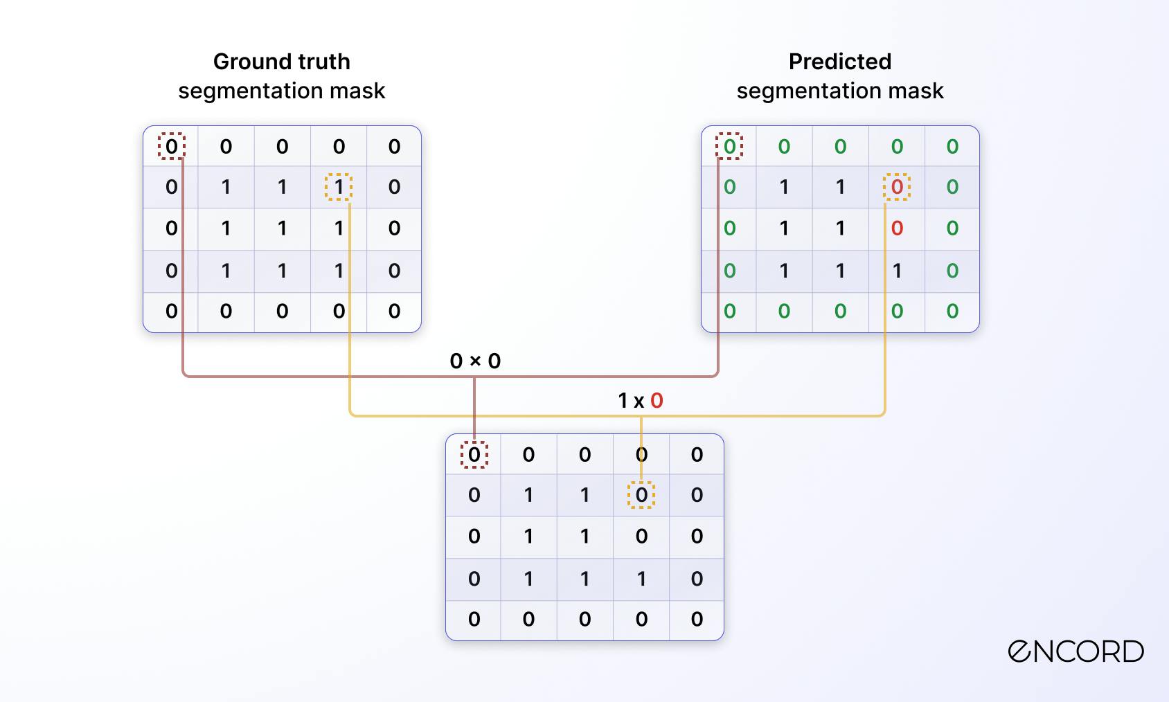
Let’s consider the previous two segmentation masks to illustrate the calculation of the mean IoU. 

• We start by identifying the number of classes, and there are two in our example:
  undefinedundefined
• Compute the IoU for each class using the formula below where: 
  undefinedundefinedundefinedundefinedundefined

IoU formula for binary classification

• For class 0, the details are given below:

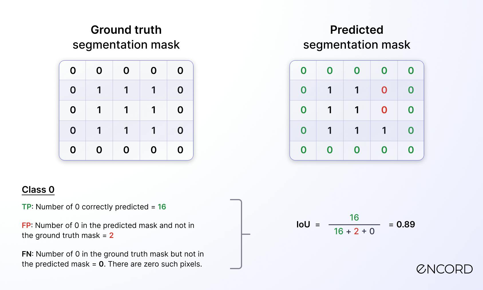
IoU calculation for class 0

• For class 1, the details are given below:

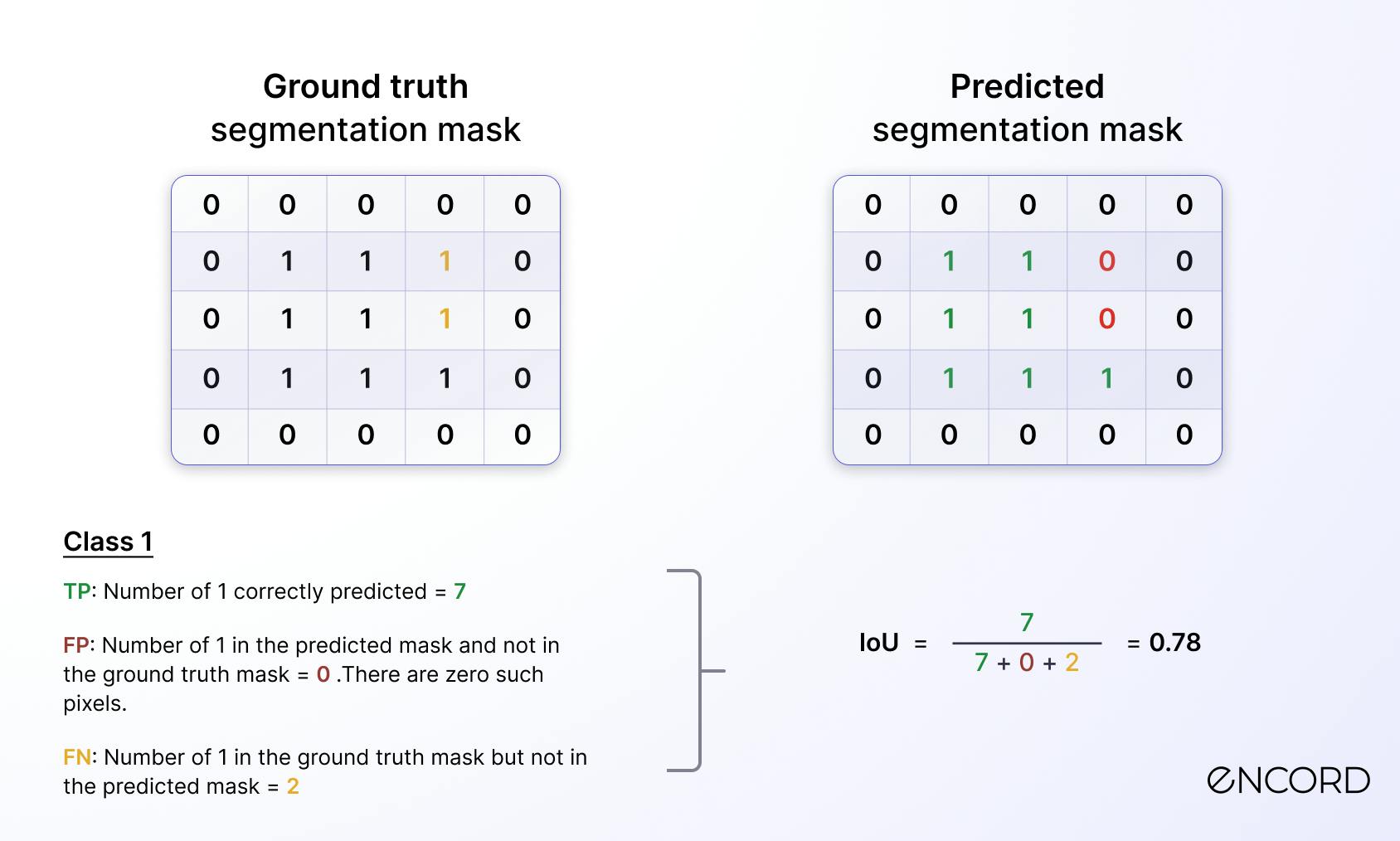
IoU calculation for class 1

• Finally, calculate the mean IoU using the formula below where n is the total number of labels: 

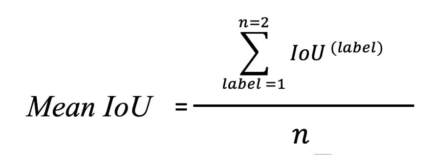
Mean IoU formula for our scenario

The final result is Mean IoU = (0.89 + 0.78) / 2 = 0.82

Dice Coefficient

Dice coefficient can be considered for image segmentation as what the F1-score is for the classification task. It is used to measure the similarity of the overlap between the predicted segmentation and the ground truth.

This metric is useful when dealing with an imbalanced dataset or when spatial coherence is important. The value of the Dice coefficient ranges from 0 to 1 when 0 means no overlap and 1 means perfect overlap. 

Below is the formula to compute the Dice Coefficient:

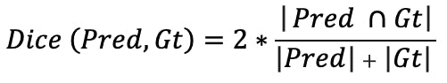
Dice Coefficient formula 

• Pred is the set of model predictions  
• Gt is the set of ground truth.

Now that you have a better understanding of what the dice coefficient is, let’s compute it using the two segmentation masks above. 

First, compute an element-wise product (intersection):

Element-wise product 

Then, calculate the sum of the elements in the previously generated matrix, and the result is 7.

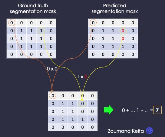
Sum of elements in the intersection mask 

 Performs the same sum computation on both the ground truth and the segmentation masks. 

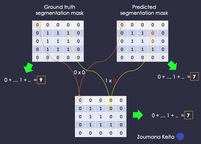
Sum of elements in all the masks 

Finally, compute the Dice coefficient from all the above scores. 

Dice = 2 x 7 / (9 + 7) = 0.875

Dice coefficient is very similar to the IoU. They are positively correlated. To understand the difference between them, please read the following stack exchange answer to dice-score vs IoU. 

Pixel-wise Cross Entropy

Pixel-wise cross entropy is a commonly used evaluation metric for image segmentation models. It measures the difference between the predicted probability distribution and the ground truth distribution of pixel labels.

Mathematically, pixel-wise cross entropy can be expressed as:

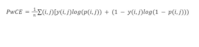
Where N is the total number of pixels in the image, y(i,j) is the ground truth label of the pixel (i,j), p(i,j) is the predicted probability of the pixel (i,j).

The pixel-wise cross entropy loss penalizes the model for making incorrect predictions and rewards it for making correct ones. A lower cross entropy loss indicates better performance of the segmentation model, with 0 being the best possible value. 

Pixel-wise cross entropy is often used in conjunction with mean intersection over union to provide a more comprehensive evaluation of segmentation models' performance.

You can read our guide to image segmentation in computer vision if you want to learn more about the fundamentals of image segmentation, different implementation approaches, and their application to real-world cases.

Wrapping up . . .

Through this article, you have learned different metrics such as mean average precision, intersection over union, pixel accuracy, mean intersection over union, and dice coefficient to evaluate computer vision models. 

Each metric has its own set of strengths and weaknesses; choosing the right metric is crucial to help you make informed decisions about evaluating and improving new and existing AI models.

Ready to improve your computer vision model performance? 

Sign-up for an Encord Free Trial: The Active Learning Platform for Computer Vision, used by the world’s leading computer vision teams. 

AI-assisted labeling, model training & diagnostics, find & fix dataset errors and biases, all in one collaborative active learning platform, to get to production AI faster. Try Encord for Free Today.  

Want to stay updated?

Follow us on Twitter and LinkedIn for more content on computer vision, training data, and active learning.

Join our Discord channel to chat and connect.

Computer Vision Model Performance FAQs

Why is the performance of a model important?

Poor model performance can lead the business to make wrong decisions hence having a bad return on investment. Better performance can ensure the effectiveness of applications relying on the models’ prediction. 

Which metrics are used to evaluate the performance of a model?

Several metrics are used to evaluate the performance of a model, and each one has its pros and cons. 

Accuracy, recall, precision, F1-score, and Area Under the Receiver Operating Characteristic Curve (AUC-ROC) are commonly used for classifications. Whereas Mean Squared Error (MSE), Mean Absolute Error (MAE), Root Mean Squared Error (RMSE), and R-Squared are used for regression tasks. 

Which model performance metrics are appropriate to measure the success of your model?

The answer to this question depends on the problem being tackled and also the underlying dataset. All the metrics mentioned above can be considered depending on the use case. 

How does accuracy affect the performance of a model?

Accuracy is easy to understand, but it should not be used as an evaluation metric when dealing with an imbalanced dataset. The result can be misleading because the model will always predict the majority class in inference mode. 

How are the performance metrics calculated?

Different approaches are used to compute performance metrics and the major ones for classification, image detection, and segmentation are covered in the article above.